is a language and environment for statistical computing and graphics.
Provides a wide variety of statistical (linear and nonlinear modelling, classical statistical tests, time-series analysis, classification, clustering, etc.) and publication-quality graphical techniques. And many more!
FREE (under GNU-GPL license).
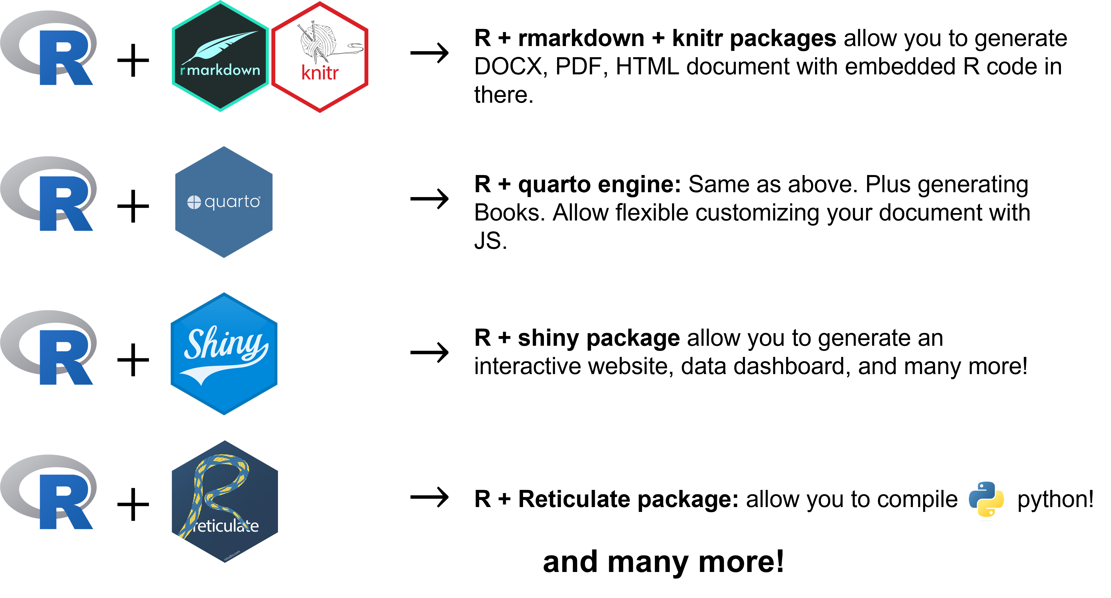
Rstudio is an integrated development environment (IDE) of R
Provides extensible environments for compiling other languages (e.g. Python, Shell, LaTeX, etc.) and engines (e.g. knitr, Jupyter, quarto, etc.)
FREE.
R vs RStudio (2)
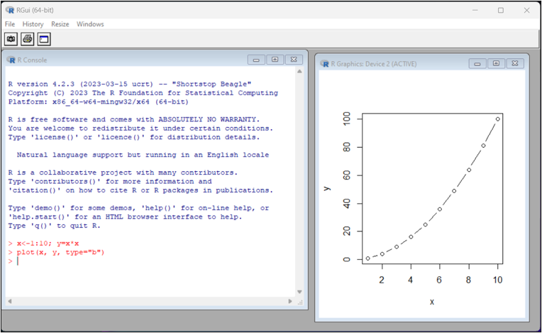
Normal R GUI
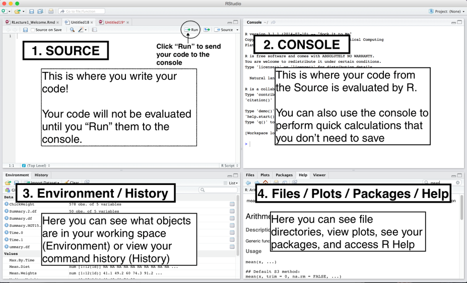
RStudio user interface and its components
R: versatility
Loading R libraries (1)
Common way to load library
library(tidyverse)
Loading R libraries (2)
More efficient way to load multiple libraries at once with pacman:
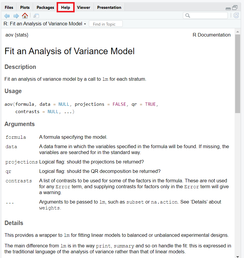
Accessing Help & Documentation in RStudio
RStudio provides built-in documentation of all functions you have installed from libraries. For example, you would like to access documentation page of function aov, simply type in the console as follows:
help(aov)# or ?aov
You can access this documentation from the Help pane. The documentation includes an explanation of the arguments, background theorem, and references for the function aov.
Tip
There are 2 recommended repositories allow you to access all documentation online, RDocumentation.org and rdrr.io. These repositories contain all the documentation for all the functions available in R, even if you have never installed it!
Data types
R has 5 data types:
Character
a <-c("May", "June", "July")class(a)
[1] "character"
Numeric
b <-c(-2.25, -1.5, 0, 1.0, 2.75, 3/4)class(b)
[1] "numeric"
Integer
c <-as.integer(b)c
[1] -2 -1 0 1 2 0
class(c)
[1] "integer"
Logical
d <-c(TRUE, FALSE, TRUE, FALSE)class(d)
[1] "logical"
Complex
e <-1+4iclass(e)
[1] "complex"
Info
R provides many functions to examine features of vectors and other objects, for example
class() - what kind of object is it?
length() - how long is it? What about two dimensional objects?
Data structure (1)
Vectors
is a row of strings (can be numbers, characters, logicals , or mix of it), and also known as a 1-dimensional array. R uses function c to declare vectors:
x <-c(1, 4, 6, 8, 10)# Inspect vectorx
[1] 1 4 6 8 10
# Access element in vectorx[2]
[1] 4
# Calculating vectorsum(x)
[1] 29
# Add another vectory <-c(2, -2, 4, 9, 0.5)y
[1] 2.0 -2.0 4.0 9.0 0.5
# Calculating vectorz <- x + yz
[1] 3.0 2.0 10.0 17.0 10.5
Matrices
is a 2-dimensional array, we use the function matrix to declare matrix in R as follow.
# Accessing element in 1st row, 2nd column of the matrixmat[1,2]
[1] 4
# Multiply matrix by 10mat*10
     [,1] [,2]
[1,]   90   40
[2,]   20   50
[3,]   30   60
# Replace value in 3rd row, 1st column of the matrix to 20mat[3,1] <-20mat
     [,1] [,2]
[1,]    9    4
[2,]    2    5
[3,]   20    6
Data structures (2)
Data frames
A data frame is a matrix in which rows and columns are named. A data frame is more flexible and compatible for further data manipulation and export as a spreadsheet. Also, data frame can be calculated like matrix.
# Create a data framet <-data.frame(name =c("gene1", "gene2", "gene3", "gene4"),cond_1 =c(20, 18, 0, 0),cond_2 =c(1, 2, 100, 120))# Access element in data framet[4, 3]
[1] 120
# See how many rows and columns in the data framedim(t)
[1] 4 3
# See what type of data format in each columnstr(t)
'data.frame':   4 obs. of  3 variables:
 $ name  : chr  "gene1" "gene2" "gene3" "gene4"
 $ cond_1: num  20 18 0 0
 $ cond_2: num  1 2 100 120
Lists
List is a complex object that can store all data types and structures, even list within list!
## Access the 2nd child element of the 3rd structure of the listL1[[3]][2]
[1] 0.25
# Calculating the listL1$five *10
[1] 0.0 2.5 5.0 7.5 10.0
Data frames (1)
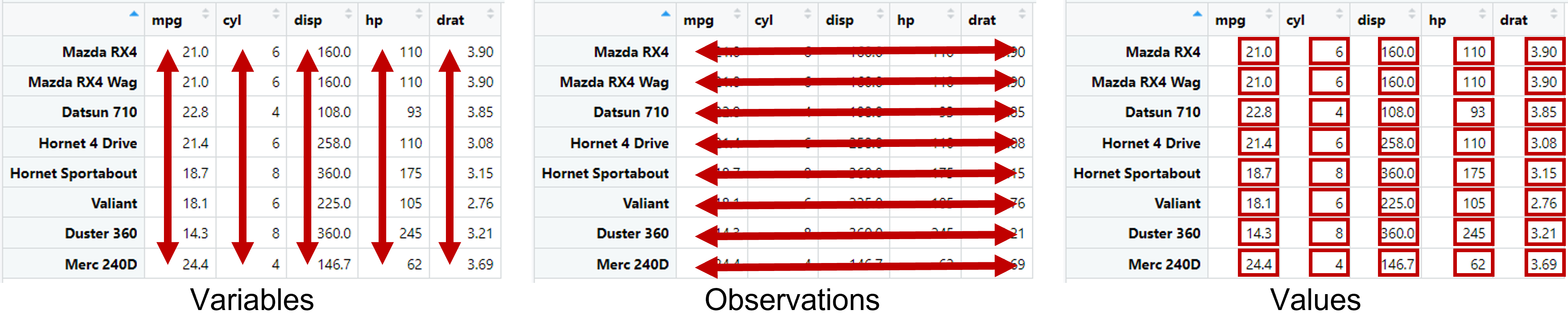
Data frame is a key data structure in R and statistics.
Each row represents observation (genes, protein, taxon, name)
Each column represents variable (measures, treatments, characteristics) of the observation
Each value in a cell represents each data point.
Structure of data frame. Redraw from R for Data Science 2nd edition (Hadley Wickham & Garrett Grolemund).
Data frames (2)
We’ll show structure of the data frames in 2 formats; wide and long formats, using airquality dataset.
Wide format
dt_wide <- datasets::airquality# Show how the data looks likehead(dt_wide)
Ozone
Solar.R
Wind
Temp
Month
Day
41
190
7.4
67
5
1
36
118
8.0
72
5
2
12
149
12.6
74
5
3
18
313
11.5
62
5
4
NA
NA
14.3
56
5
5
28
NA
14.9
66
5
6
Human-readable data frame
Elegance
Easy to see all values in each observation
One observation is one row
May incompatible for some plots in ggplot2
Long format
dt_long <- datasets::airquality %>%pivot_longer(!c(Day, Month))# Show how the data looks likehead(dt_long)
Month
Day
name
value
5
1
Ozone
41.0
5
1
Solar.R
190.0
5
1
Wind
7.4
5
1
Temp
67.0
5
2
Ozone
36.0
5
2
Solar.R
118.0
Machine-readable data frame
Simple
Each observation can be more than one row
Compatible to include with metadata table (if any)
ggplot2 ❤️long-format data frame
Managing data frames with dplyr
We can handle data frames with base R, but when you are working with a large data set, speed matters. The dplyr package provides a “grammar” (especially verbs) for data manipulation and for editing data frames.
Frequently used dplyr verbs:
glimpse: skim structure of the data, see every columns in a data frame.
select: return a subset of the columns of a data frame, using a flexible notation.
filter: extract a subset of rows from a data frame based on logical conditions.
arrange: reorder rows of a data frame.
rename: rename variables in a data frame.
mutate: add new variables/columns or transform existing variables.
summarise / summarize: generate summary statistics of different variables in the data frame, possibly within strata.
%>%: the “pipe” operator, is used to connect multiple verb actions together into a pipeline.
Common dplyr Function Properties
The first argument must be a data frame to process.
The subsequent arguments describe what to do with the data frame specified in the first argument, and you can refer to columns in the data frame directly without using the $ operator (just use the column names).
The return result of a function is a new data frame
For example:
# Load dplyr librarylibrary(dplyr)# Load airquality datasetdt <- datasets::airqualitydt_filtered <-filter(dt, Solar.R >300)# Show how the data looks likehead(dt_filtered)
We already have data frame dt_iris from earlier practice. Now we will select columns name Species, and Petal.Width from dt and store in new variable: dt_sel
# Select columns Petal.Width and Species from dt, keep in dt_seldt_sel <-select(dt_iris, Species, Petal.Width)
The glimpse the result.
# Check the result by glimpseglimpse(dt_sel)
dplyr::filter
filter() is used to subset a data frame, retaining all rows that satisfy your conditions.
From the data set iris stored in data frame dt_iris,
Now we will filter Species ‘versicolor’.
# Filter versicolor species in dt_irisdt_versicolor <-filter(dt_iris, Species =="versicolor")# Glimpse the resultglimpse(dt_versicolor)
From dt_versicolor, filter the flowers that the Sepal.Length longer than or equal to 6
# Filter the versicolor iris that the sepal length longer than or equal to 6dt_vsc_filt <-filter(dt_versicolor, Sepal.Length >=6)
Then glimpse the result
# Glimpse the resultglimpse(dt_vsc_filt)
dplyr::arrange
arrange() orders the rows of a data frame by the values of selected columns.
In our filtered data frame dt_vsc_filt, sort the Sepal.Length column.
# Sort data frame dt_vsc_filt by sepal length column (ascendingly)dt_vsc_filt_srt <-arrange(dt_vsc_filt, Sepal.Length)
Then, sort the Petal.Length descendingly.
# Sort data frame dt_vsc_filt descendingly by petal length columndt_vsc_filt_srt <-arrange(dt_vsc_filt, desc(Petal.Length))
Glimpse the result
glimpse(dt_vsc_filt_srt)
dplyr::rename
rename() changes the names of individual variables using new_name = old_name syntax.
From sorted and filtered data frame dt_vsc_filt_srt, we will rename 2 columns, from Sepal.Length and Petal.Length, to SL and PL, respectively. Then save to the new data frame dt_vsc_renamed.
# Rename column from Sepal.Length to SL, and Petal.Length to PL, then save to the new data frame dt_vsc_renameddt_vsc_renamed <-rename(dt_vsc_filt_srt, SL = Sepal.Length,PL = Petal.Length)
dplyr::mutate
mutate() creates new columns that are functions of existing variables, as well as modify and delete columns.
From the previous data frame dt_vsc_renamed, we’ll calculate the difference between sepal length SL and petal length PL to the new column Len_Diff. This can be done with the mutate() function as follow.
# Calculate difference of sepal length and petal length, add to the new column Len_Diffdt_vsc_renamed <-mutate(dt_vsc_renamed,Len_Diff = SL - PL)
Then, use function summary() to see the distribution of the values using the column Len_Diff.
# Rough summarize the difference of sepal length and petal length
summary(dt_vsc_renamed$Len_Diff)
Expected result:
   Min. 1st Qu.  Median    Mean 3rd Qu.    Max.
    0.9     1.5     1.9     1.8     2.0     2.3
dplyr::%>%
The pipeline operator %>% (pronounce: pipe) is very handy for bundling dplyr verbs and creating complex syntax for processing data. For example:
Instead of using dplyr verbs and storing the new variables line by line, we can bundle them and use %>%. All operations associated with %>% are stored in one variable.
We loaded the iris data set to the variable iris_df.
Then rename the column name with rename() function.
Then calculate the difference of sepal length and petal length using mutate() function.
And keep the difference that are greater than 1 using filter() function.
All of these verbs are operated and store in one variable, iris_df.
dplyr::summarize
summarise() returns one row for each combination of grouping variables. It will contain one column for each grouping variable and one column for each of the summary statistics that you have specified.
We’ll load original datasets::iris to the new data frame dt2_iris.
Of these 3 species, calculate mean and standard deviation of petal length using mean() and sd(), respectively. Then calculate the standard deviation of mean (SEM) of the petal length.
Plotting is an important tool for understanding data properties, finding patterns in the data, suggesting modeling strategies for our data, and communicating what we have found in our data. Many plotting systems available in R such as:
Base graphic conventional way, same as implementing graphical visualizations in the S language. You can only draw on the plot, and append another plot to it.
Grid graphic or Grobs (graphical objects), not used to create statistical graphs per se, but are insanely useful in combining and laying out multiple graphic devices.
Lattice Plots uses lattice graphics to implement the Trellis graphics system. Also known as an improved version of Base Plot.
ggplot2 improves base and lattice graphics. The graphics are drawn using grids, which allows you to manipulate their appearance at many levels.
htmlwidgets provides a common framework for accessing web visualization tools from R. Userful for creating interactive plots for publishing on websites.
plotly is a popular javascript visualization toolkit with an R interface. It is a great tool if you want to create interactive graphics for HTML documents or websites.
Another graphic systems, ComplexHeatmap (Gu 2022), will be used in this workshop as well.
Base graphics (1)
Using library graphics, plain and simple plot functions in R is usually called R base plot. The syntax is shown as follow:
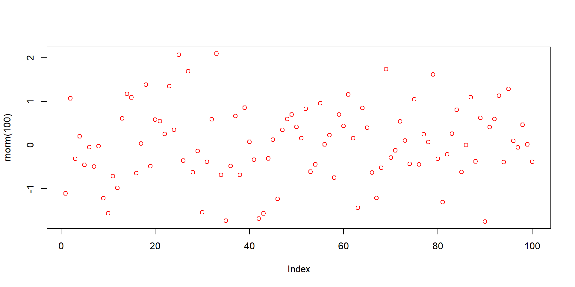
plot(rnorm(100), type ="p", col ="red")
This is a scatter plot showing 100 random numbers. Each red point indicates a data point.
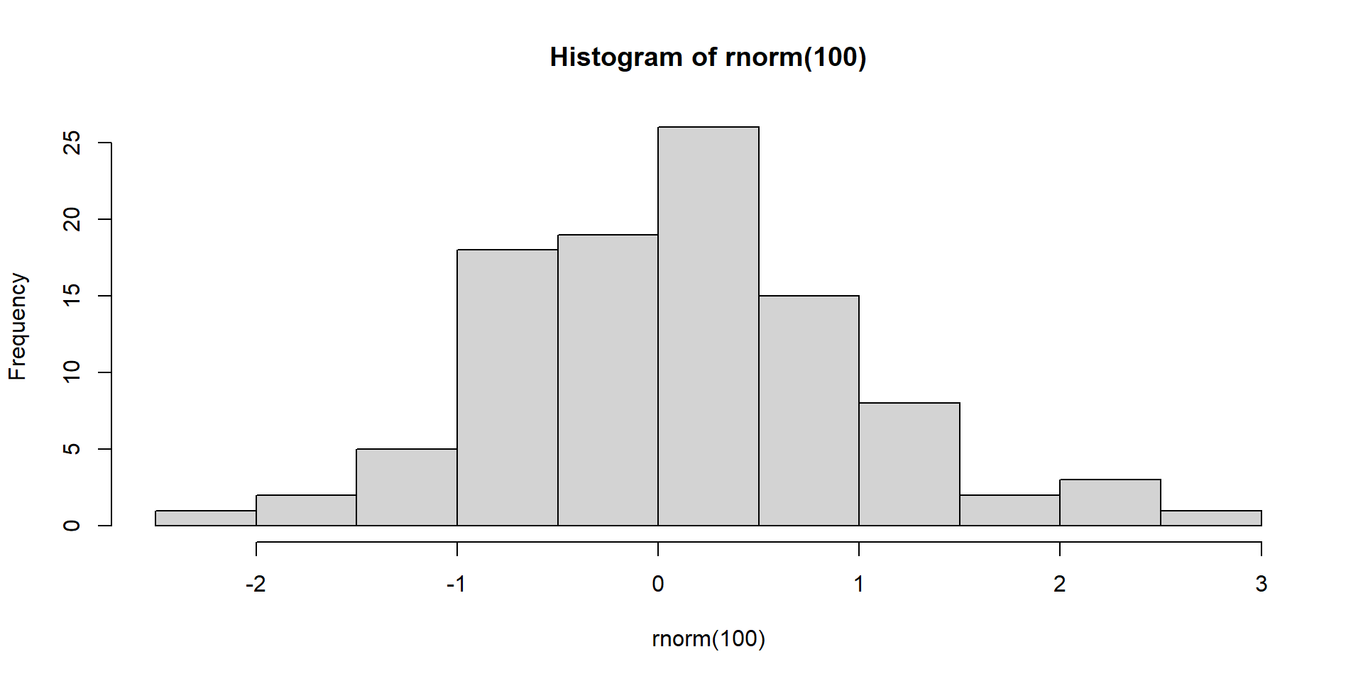
hist(rnorm(100))
Another simple plot to show the pattern of the data is histogram.
Base graphics (2)
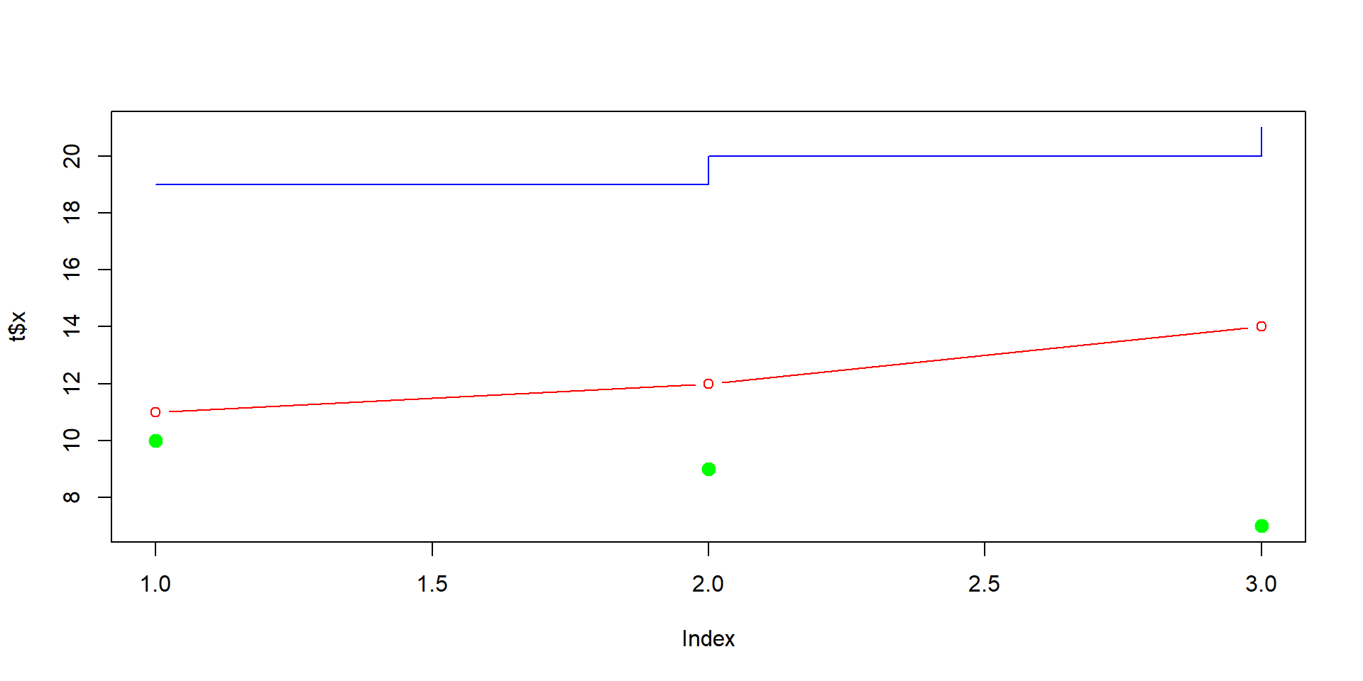
The following lines create a plot from data frame t.
# Creating a data framet <-data.frame(x =c(11,12,14), y =c(19,20,21), z =c(10,9,7))# Creating a new plotplot(t$x, type ="b", ylim =range(t), col ="red")# Adding new graphic to the plotlines(t$y, type ="s", col ="blue")# Adding another graphic to the plotpoints(t$z, pch =20, cex =2, col ="green")
Lattice graphic
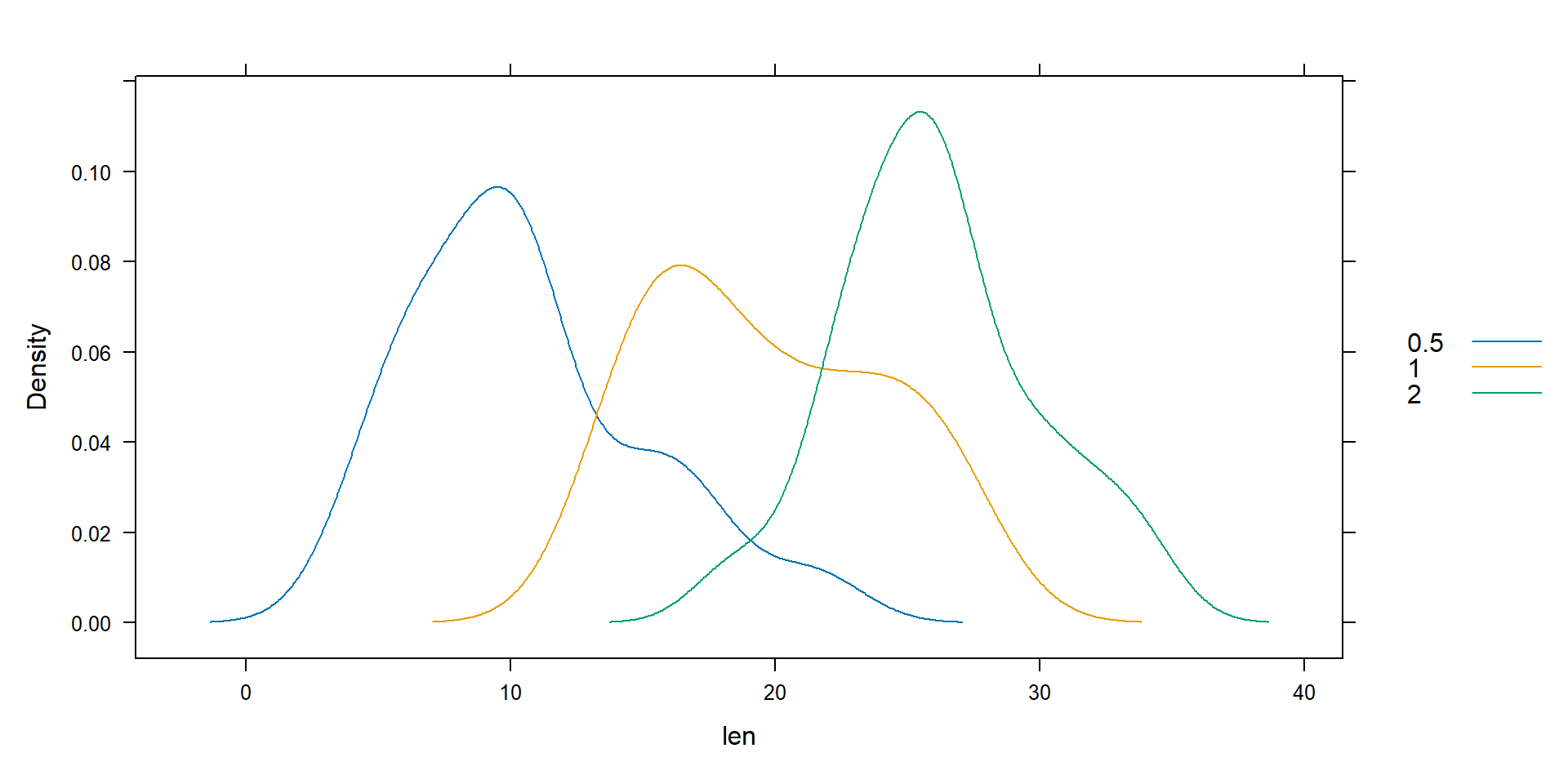
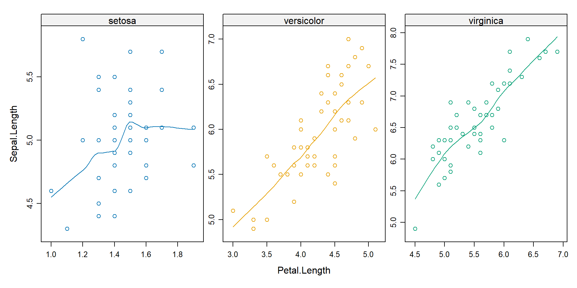
Attempts to improve R’s basic graphs by providing better presets and the ability to display multivariate relationships. In particular, the package supports the creation of grid graphs - graphs that show a variable or the relationship between variables as a function of one or more other variables.
# Load packagelibrary(lattice)# Load Toothgrowth data setToothGrowth <- datasets::ToothGrowth# Density plotdensityplot(~ len, groups = dose, data = ToothGrowth,plot.points =FALSE, auto.key =TRUE)
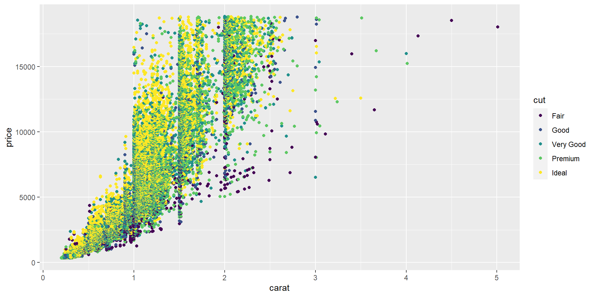
The ggplot2 package is an R package for creating graphs or plots of statistical data. With ggplot2, you can compose graphs by combining independent components based on the Grammar of Graphics.
# Load packagelibrary(ggplot2)# create scatterplot of carat vs. price, # using cut as color variableggplot(data = diamonds, aes(x = carat, y = price, color = cut)) +geom_point()
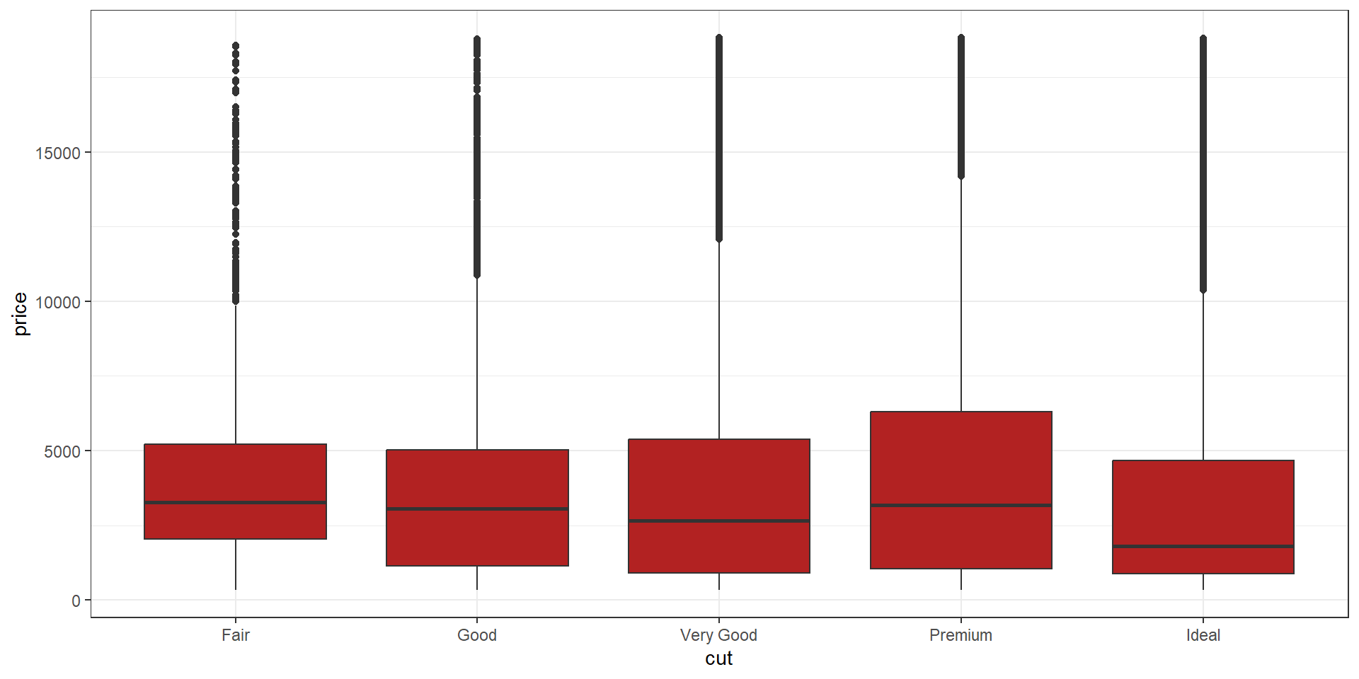
# Create scatterplot of price, grouped by cutggplot(data = diamonds, aes(x = cut, y = price)) +geom_boxplot(fill ="firebrick") +theme_bw()
We’ll mainly use ggplot2 and other graphic libraries in this workshop 🙂
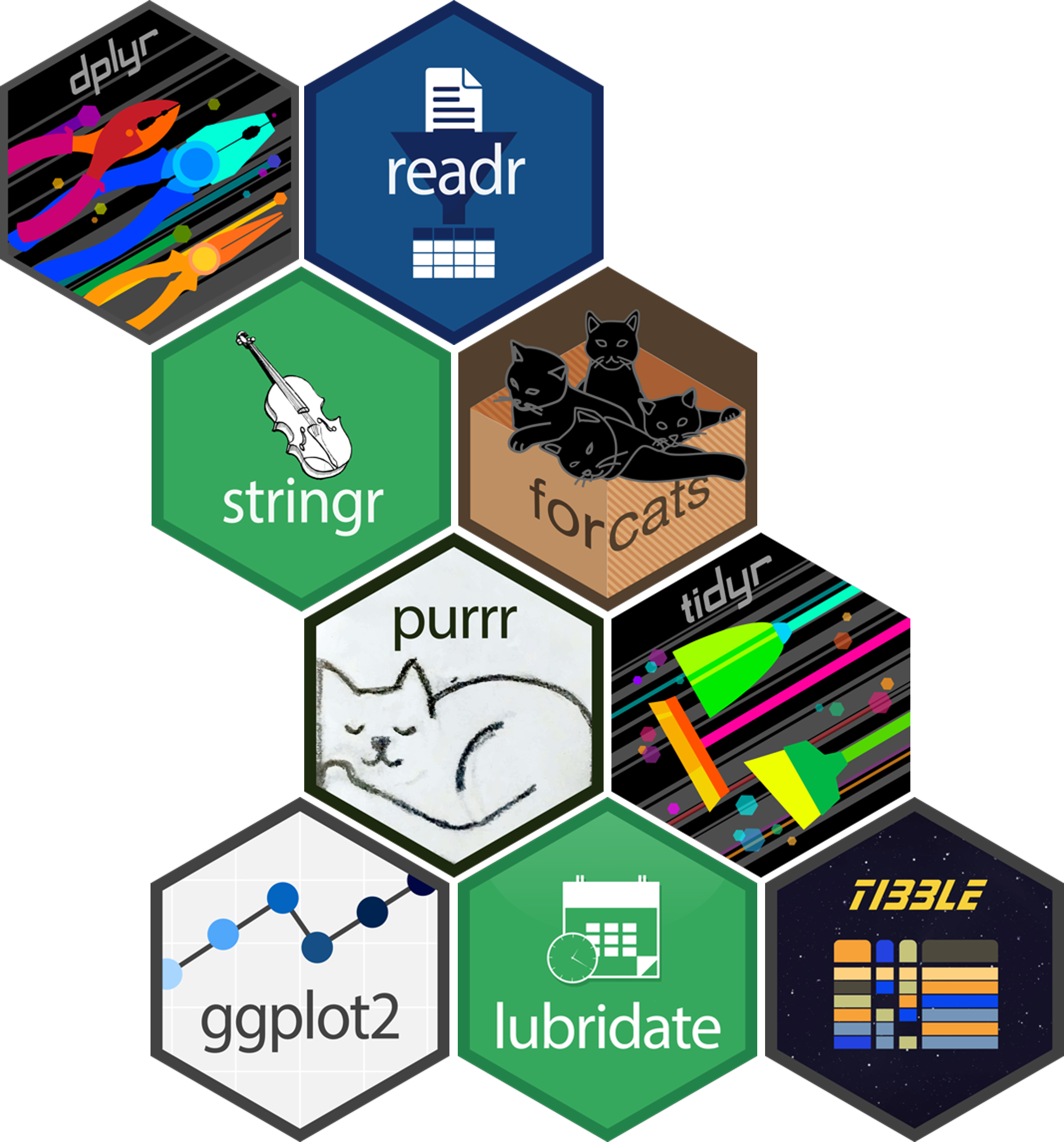
Tidyverse
Tidyverse is a collection of R packages for data science. All Tidyverse packages share the same design philosophy, grammar, and data structures. The core of Tidyverse includes packages that you will use in your daily data analysis.
# Load tidyverselibrary(tidyverse)
Core packages in Tidyverse.
References
A (very) short introduction to R: written by Torfs & Brauer, Hydrology and Quantitative Water Management Group, Wageningen University.