Grammar of Graphics
What is Grammar of Graphics
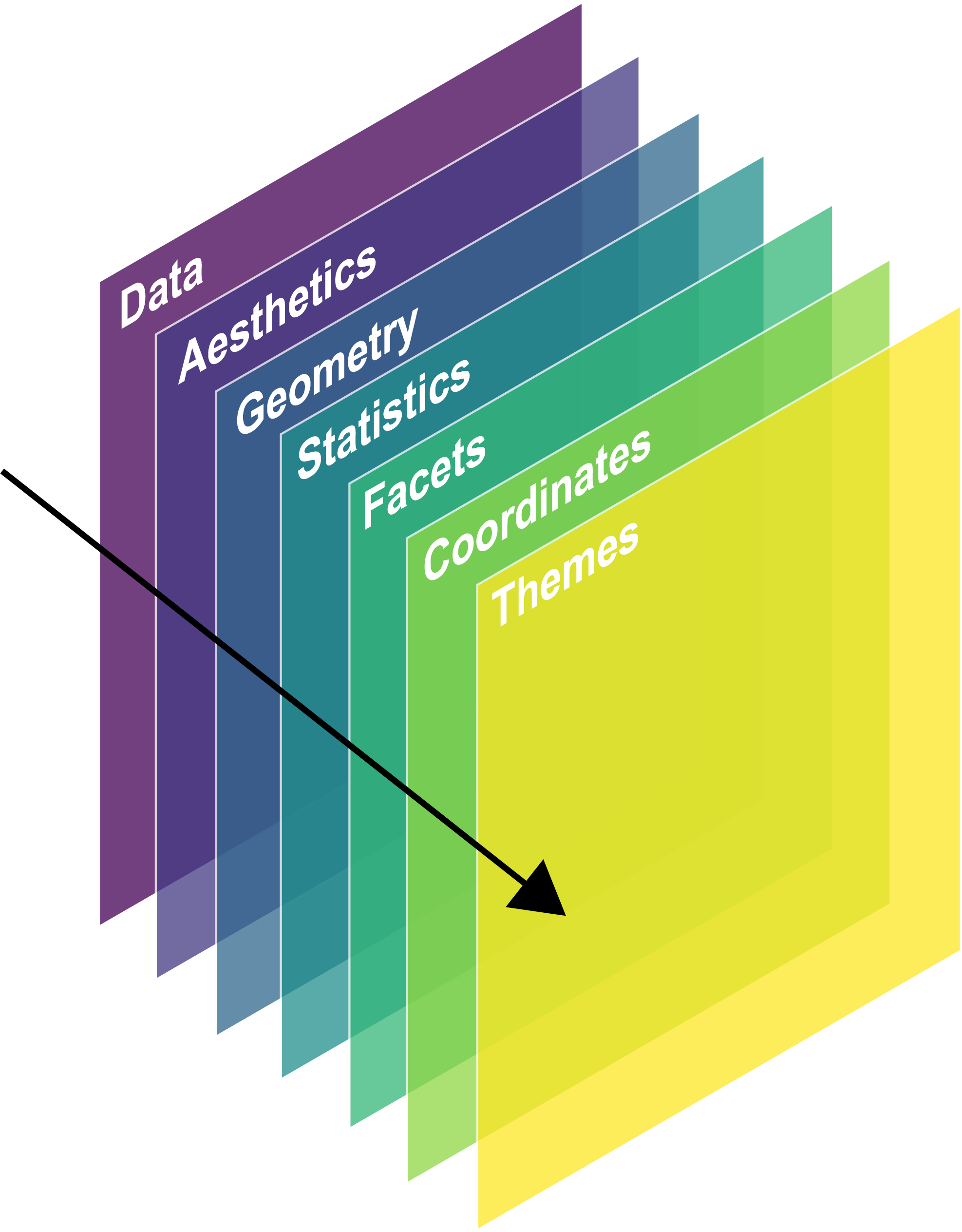
Data: Your input data (in long format)
Aesthetics: what makes your data visible, e.g., size, line color, variables to plot, fill color, line type, transparency, etc.
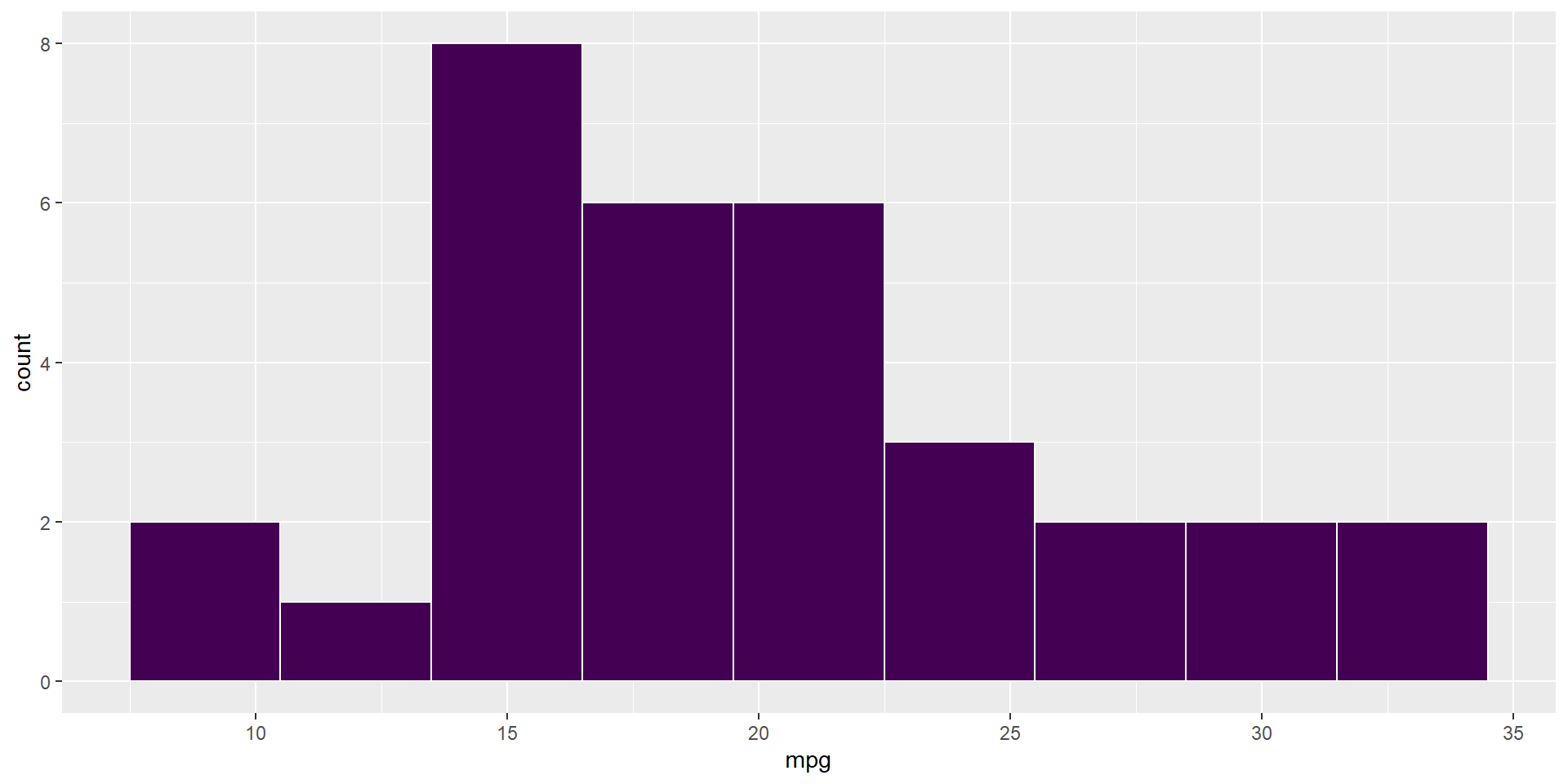
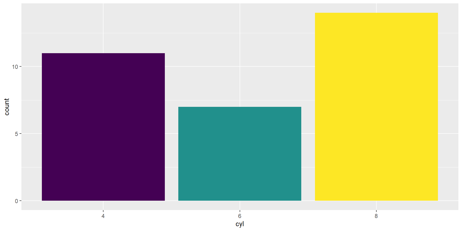
Geometry: determines the type of plot.
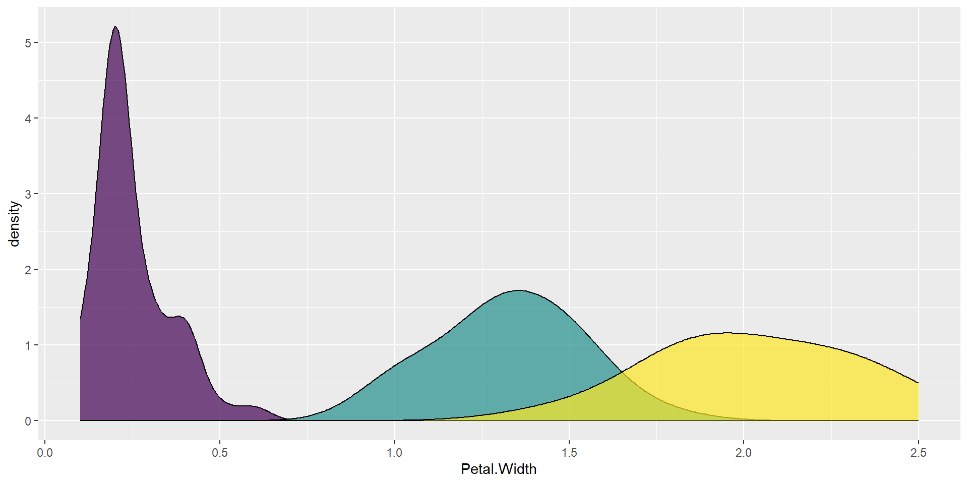
Statistics: statistical transformation of continuous data
Facets: for splitting plot into subplots.
Coordinates: Numeric systems to limit, breakdown, transform position of geometry.
Themes: Overall visual of plots and customization.
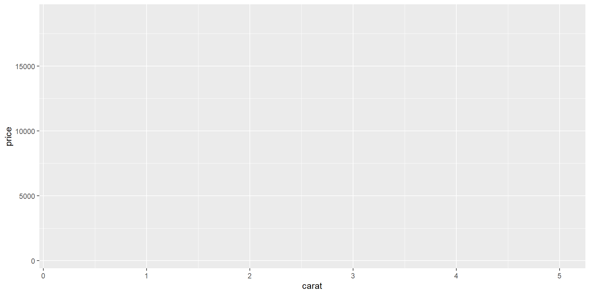
Building a plot layer-by-layer
- Load data with
ggplot()

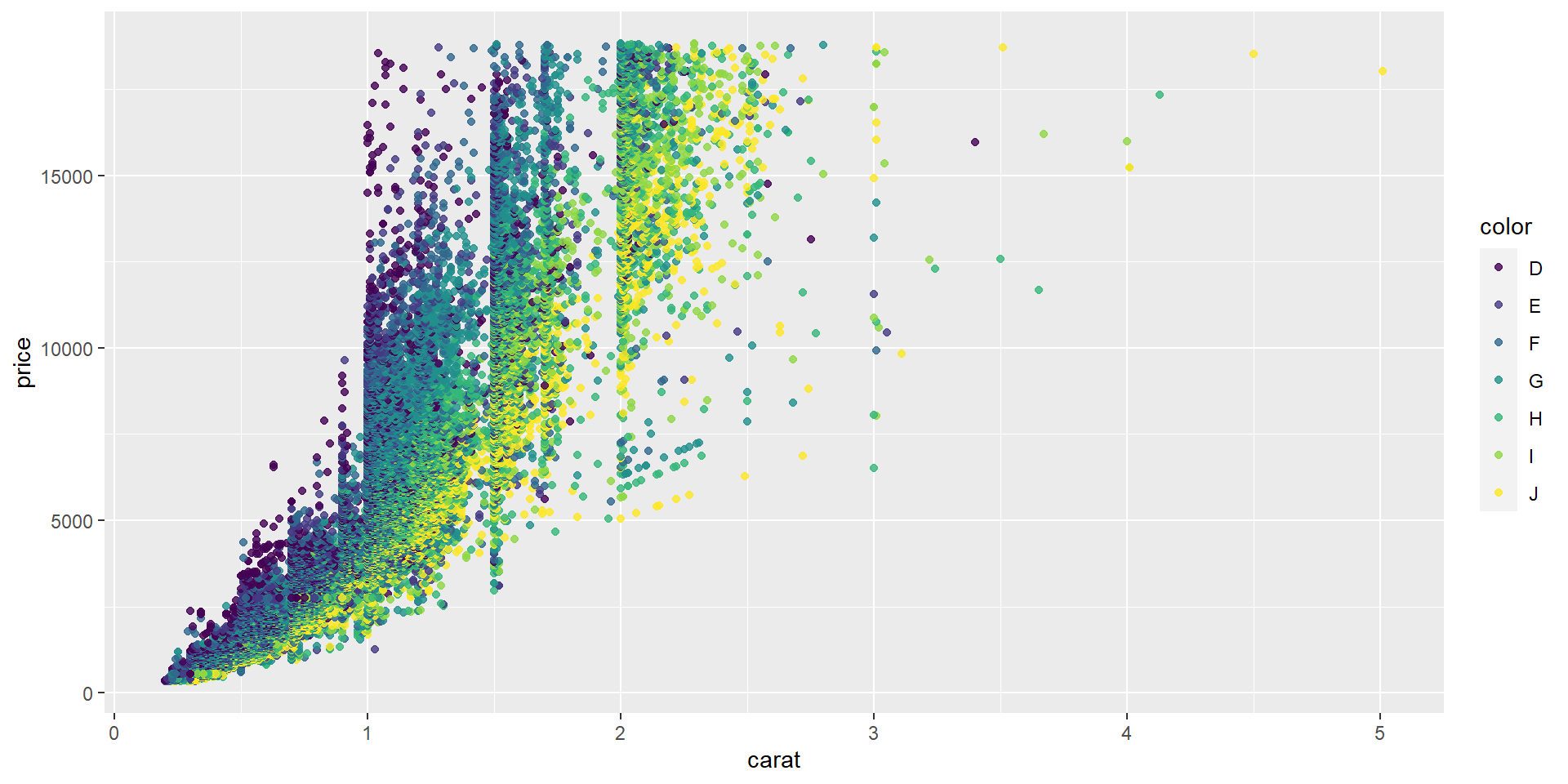
Building a plot layer-by-layer
- Add aesthetics by
aes()
Building a plot layer-by-layer
- Add geometry by
geom()
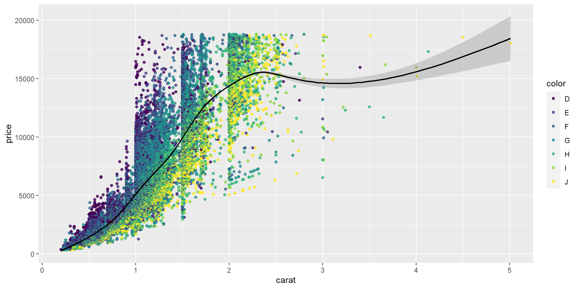
Building a plot layer-by-layer
- Add statistics
Building a plot layer-by-layer
- Add facets
Building a plot layer-by-layer
- Adding coordinates
Building a plot layer-by-layer
- Adding theme
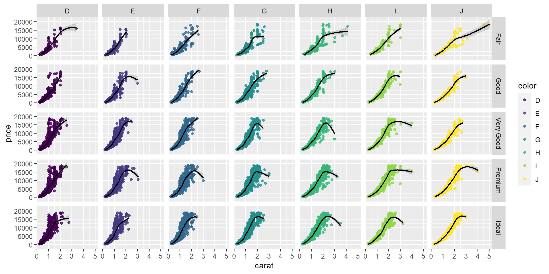
# Load library
library(ggplot2)
# Define data and global aesthetics
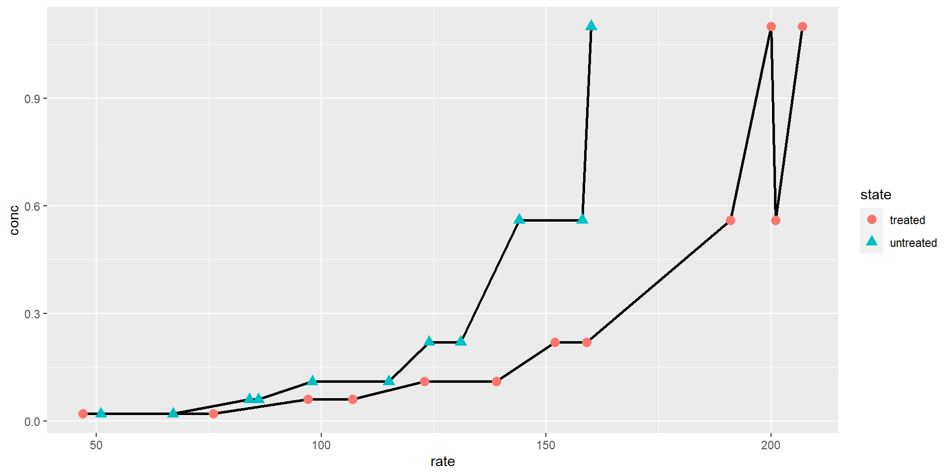
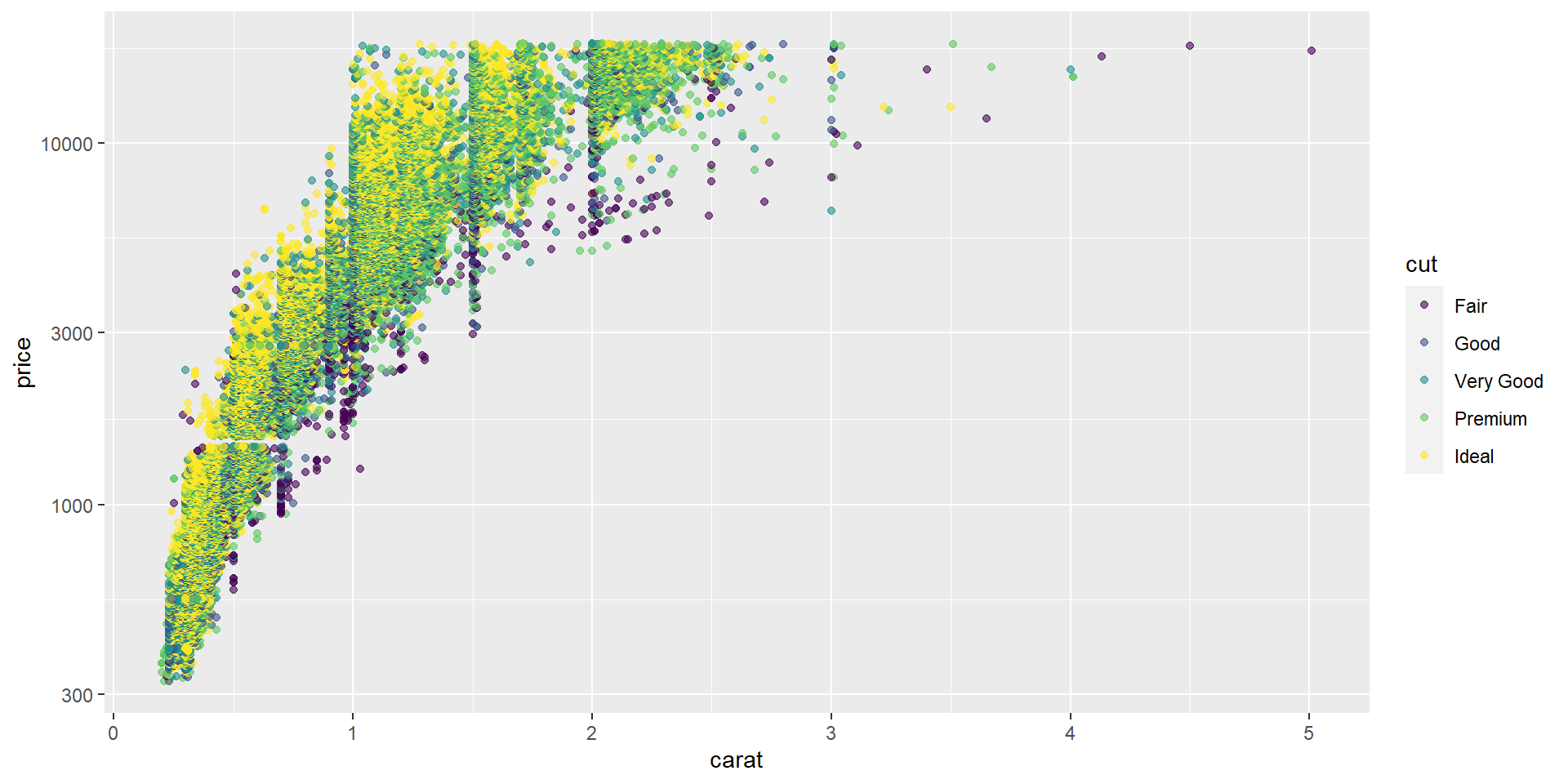
ggplot(diamonds, aes(x = carat, y = price, color = color)) +
geom_point(alpha = 0.8) +
stat_smooth(color = "black", linewidth = 0.8) +
facet_grid(cut ~ color) +
scale_y_continuous(breaks = seq(from = 0, to = 20000, by = 10000)) +
theme_bw()
Aesthetics
Aesthetics
aes()describe how variables map to visual properties or aesthetics.The position of data points are described by values from
xandyshape, size, or color styles can also be specified in
aes().
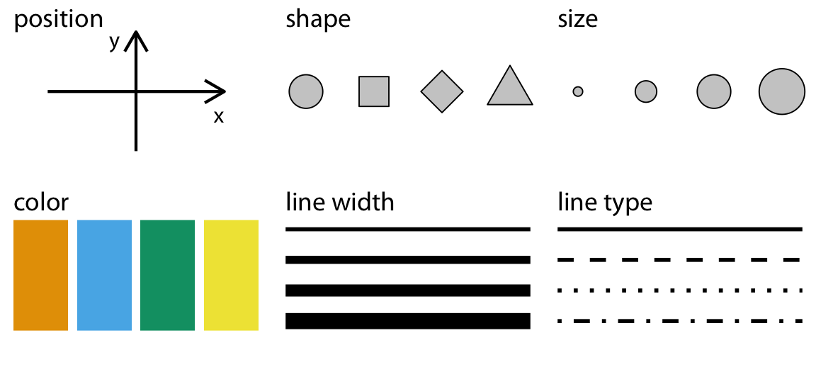
Commonly used aesthetics in data visualization: position, shape, size, color, line width, line type. Figure from Wilke (2019)
Geoms
Frequently used geoms (Explore more plot in R Graph Gallery: https://r-graph-gallery.com)


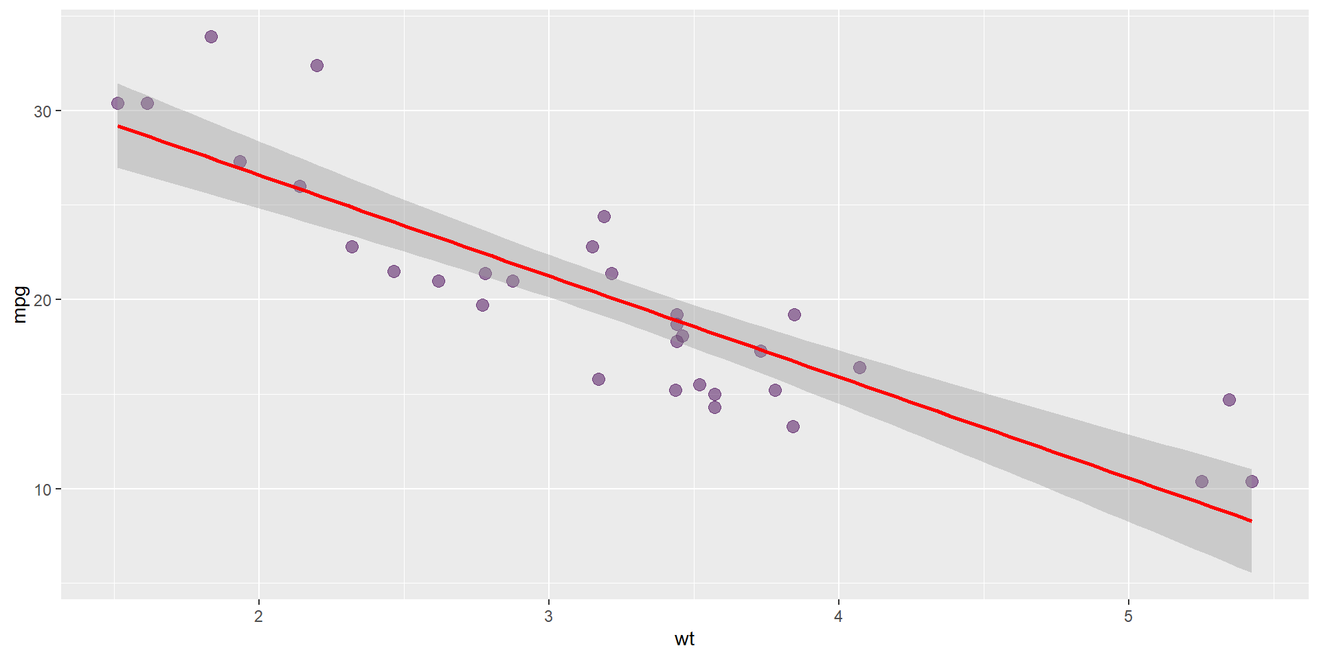
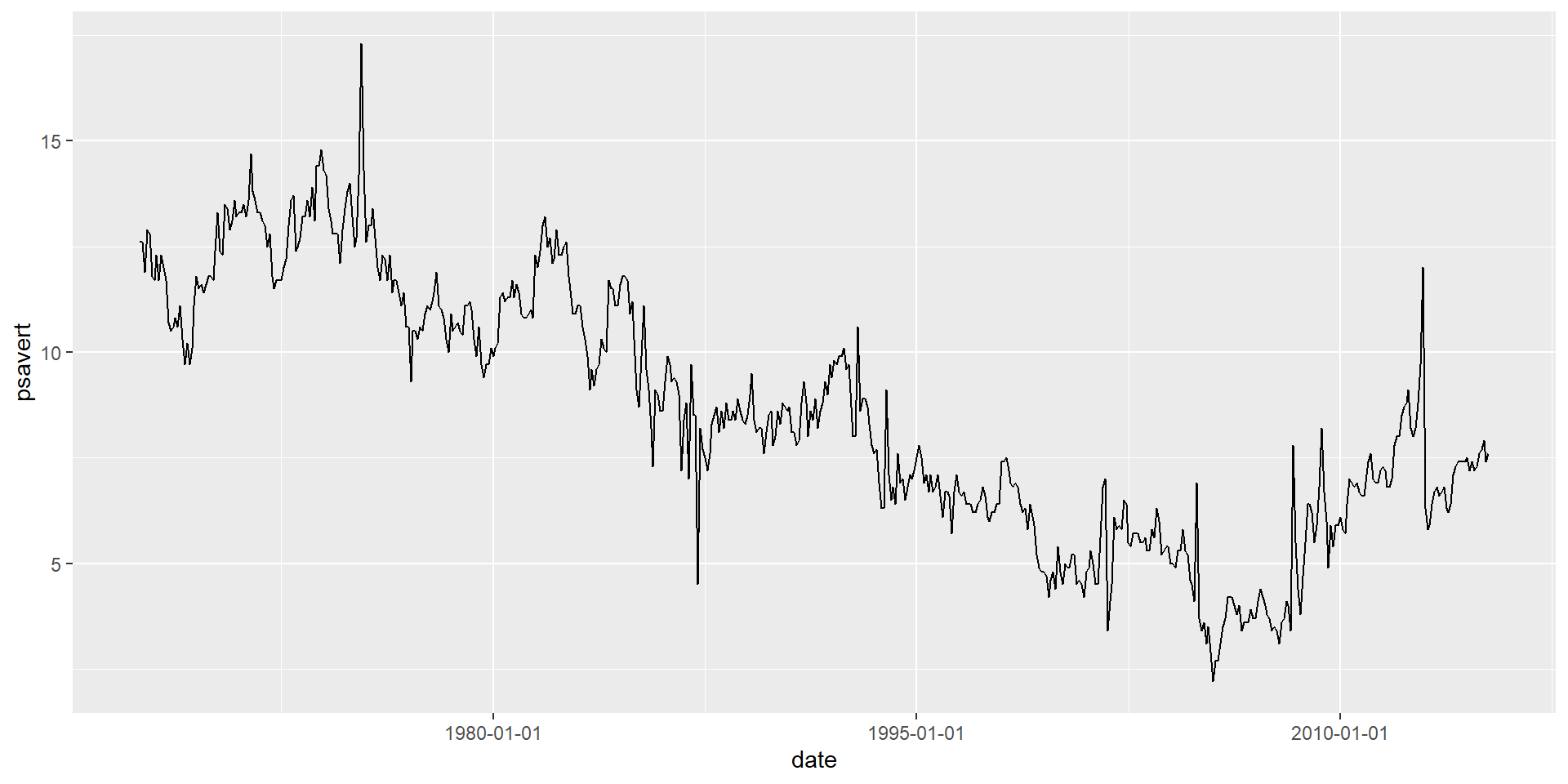
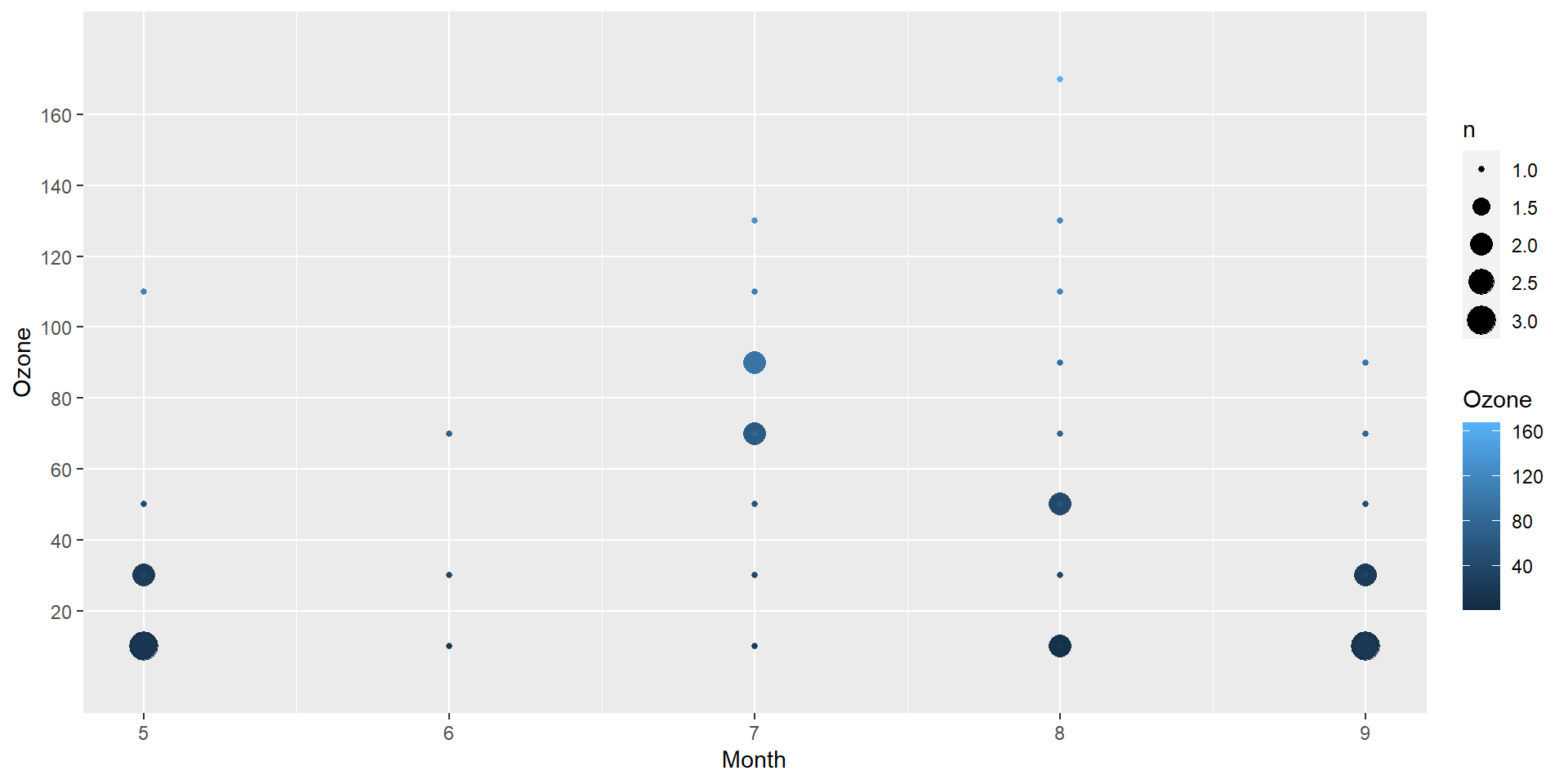
Position scales and axes
Numeric position scales
- Limit
Position scales and axes
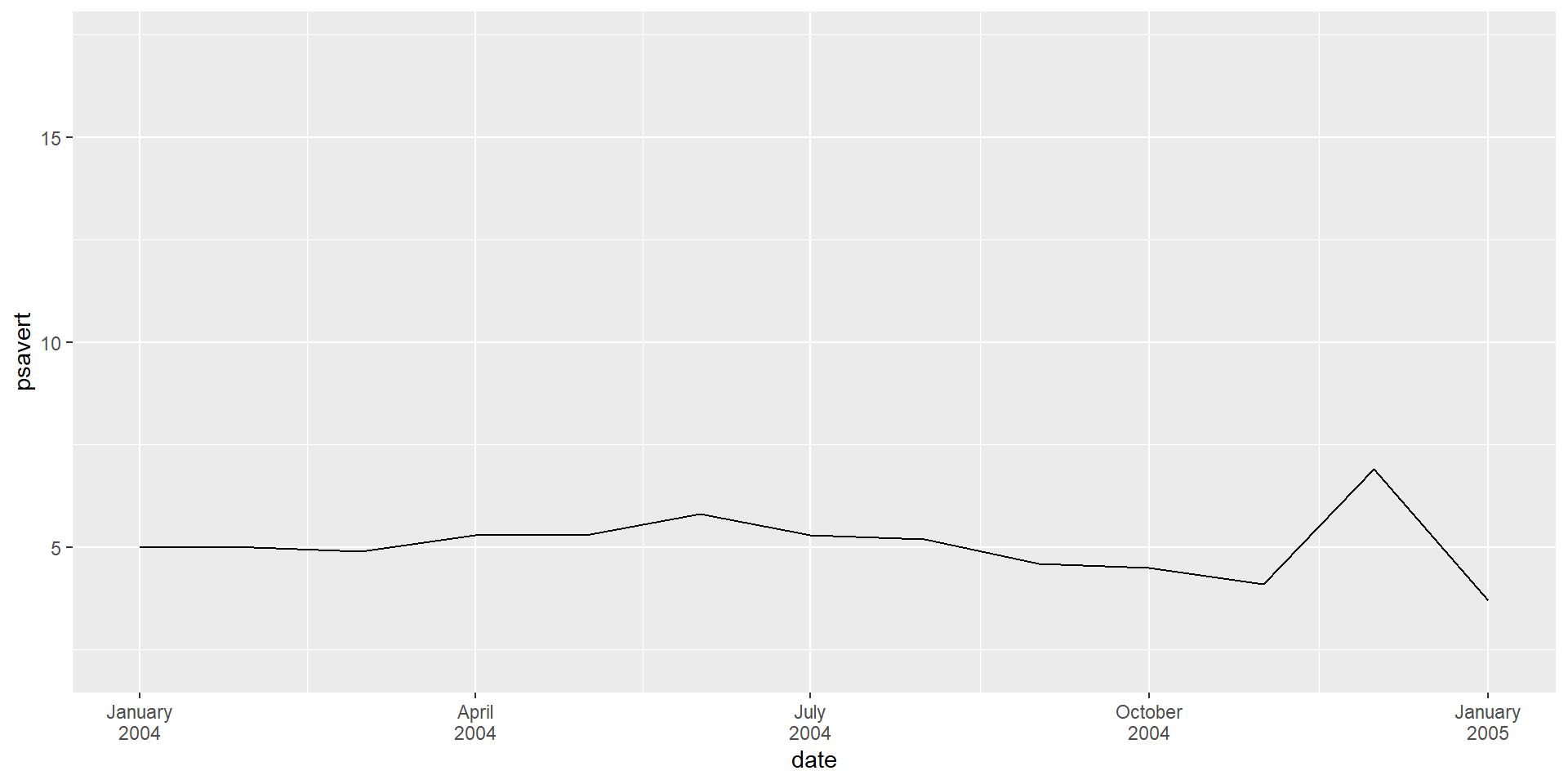
Numeric position scales (2)
- Expand
Position scales and axes
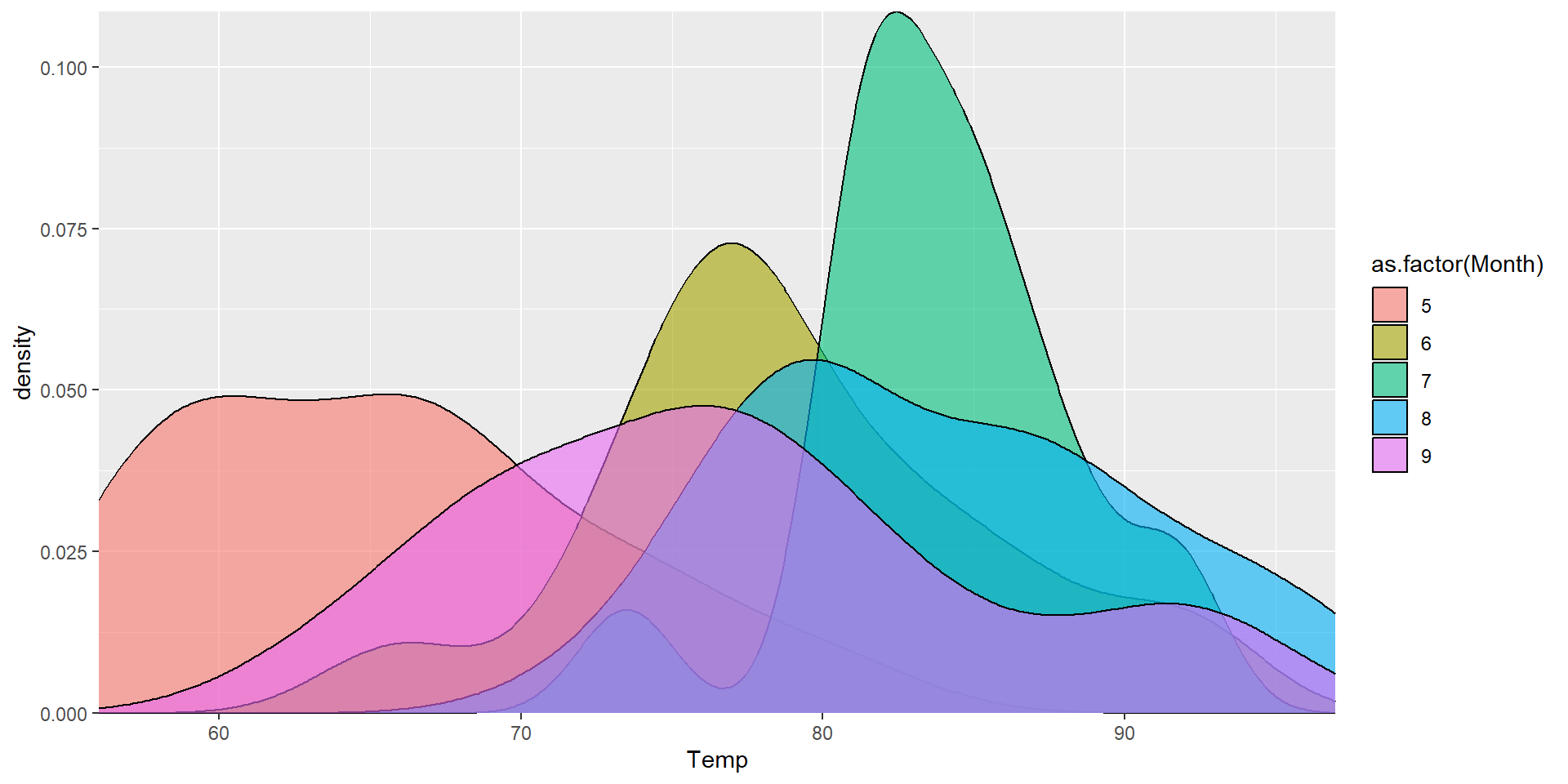
Date-time position scale
Date scales behave like numeric scales, it’s ordinal, but is often more convenient to use the date_labels argument with the predefined formats. More available formatting strings: https://ggplot2-book.org/scales-position.html#sec-date-labels.
Position scales and axes
Binned position scales
Color scales and legends
Color blindness
Available color palettes from package colorBlindness.
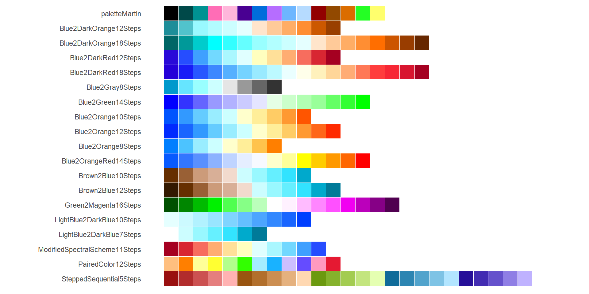
More information on R colorBlindness package: https://cran.r-project.org/web/packages/colorBlindness/vignettes/colorBlindness.html
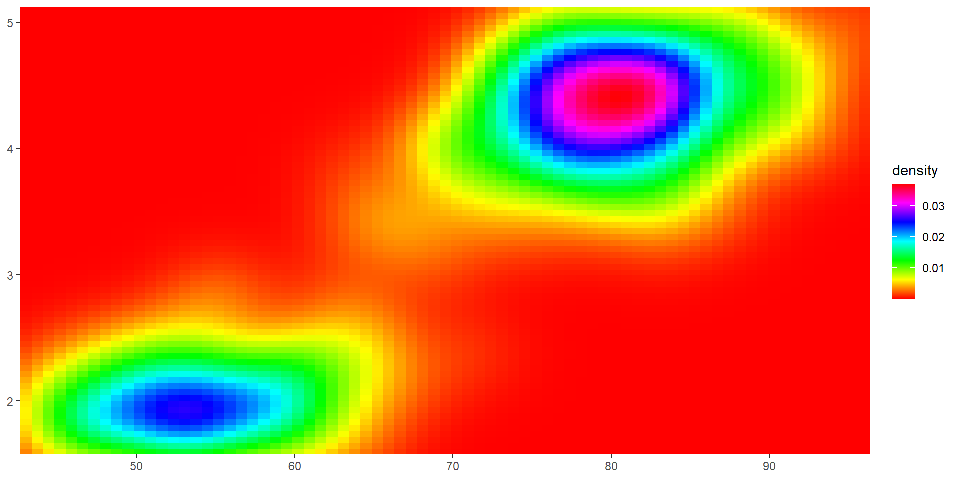
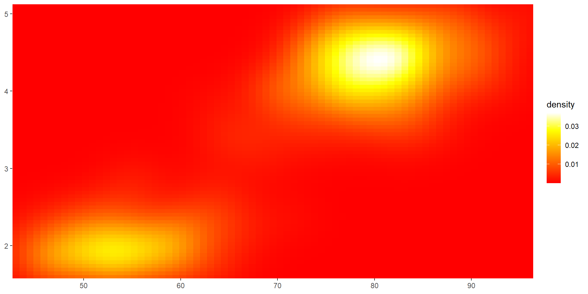
Color scales and legends
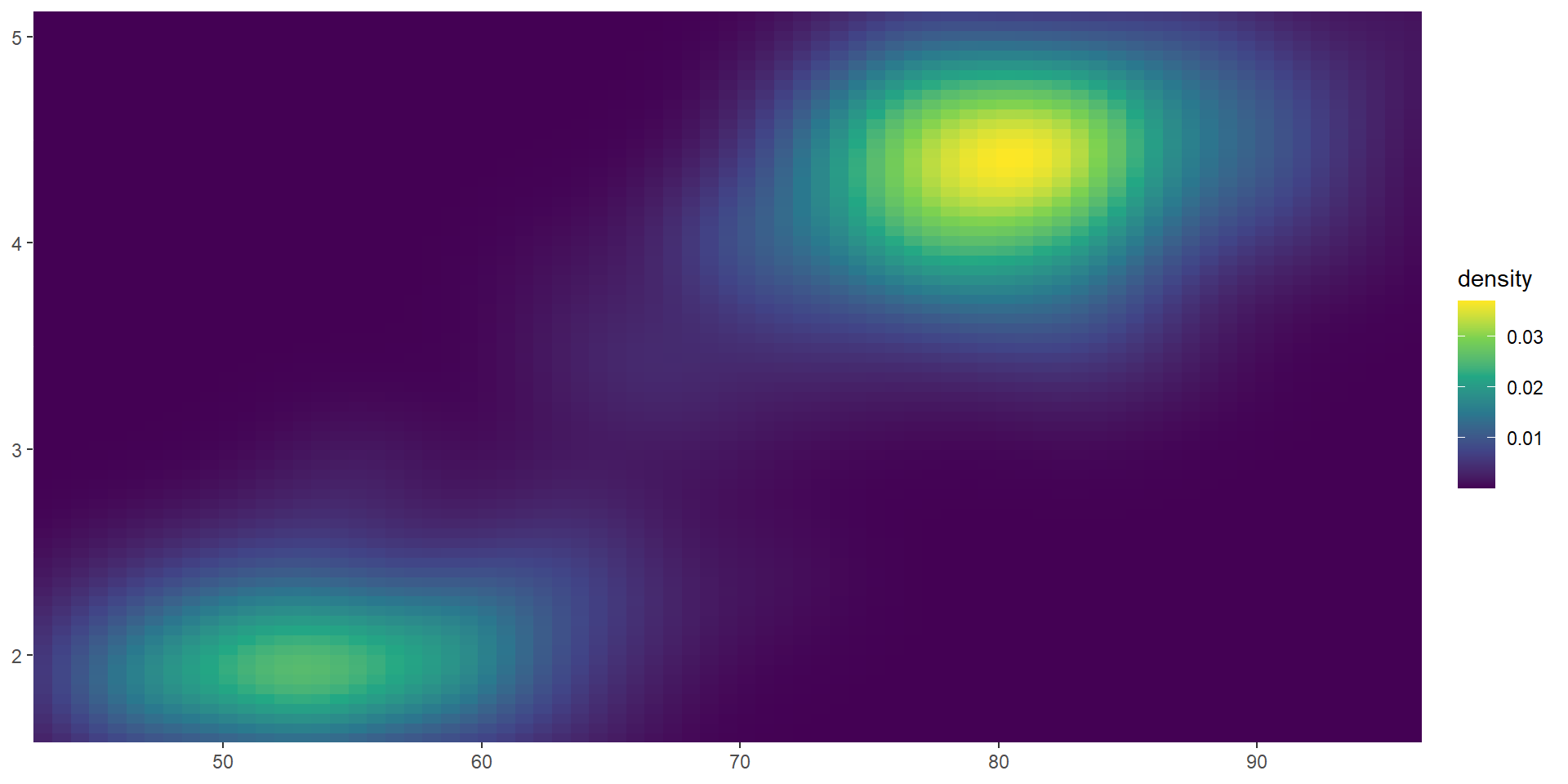
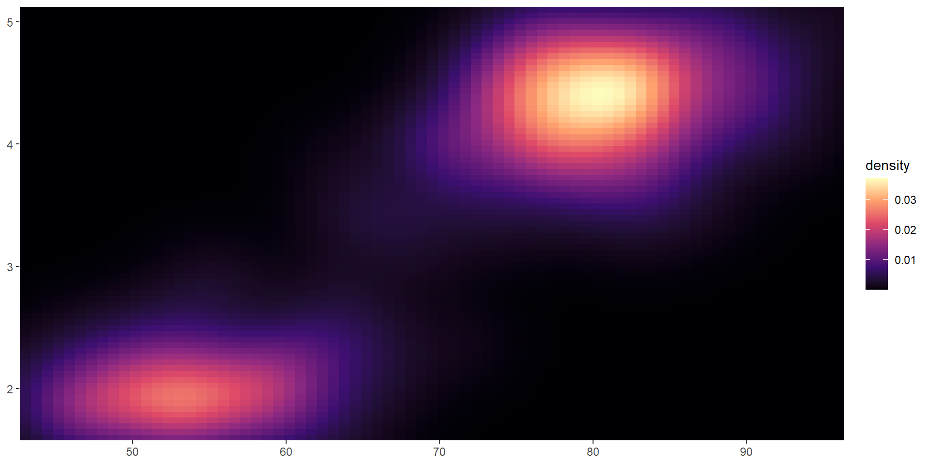
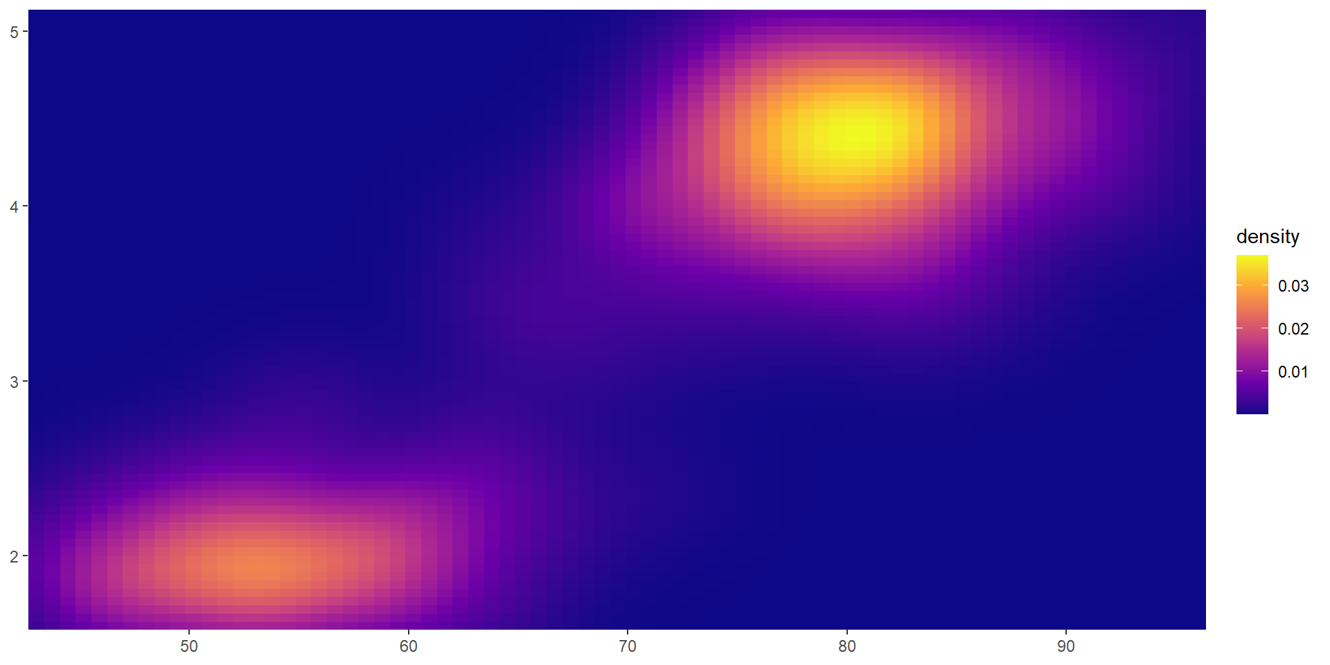
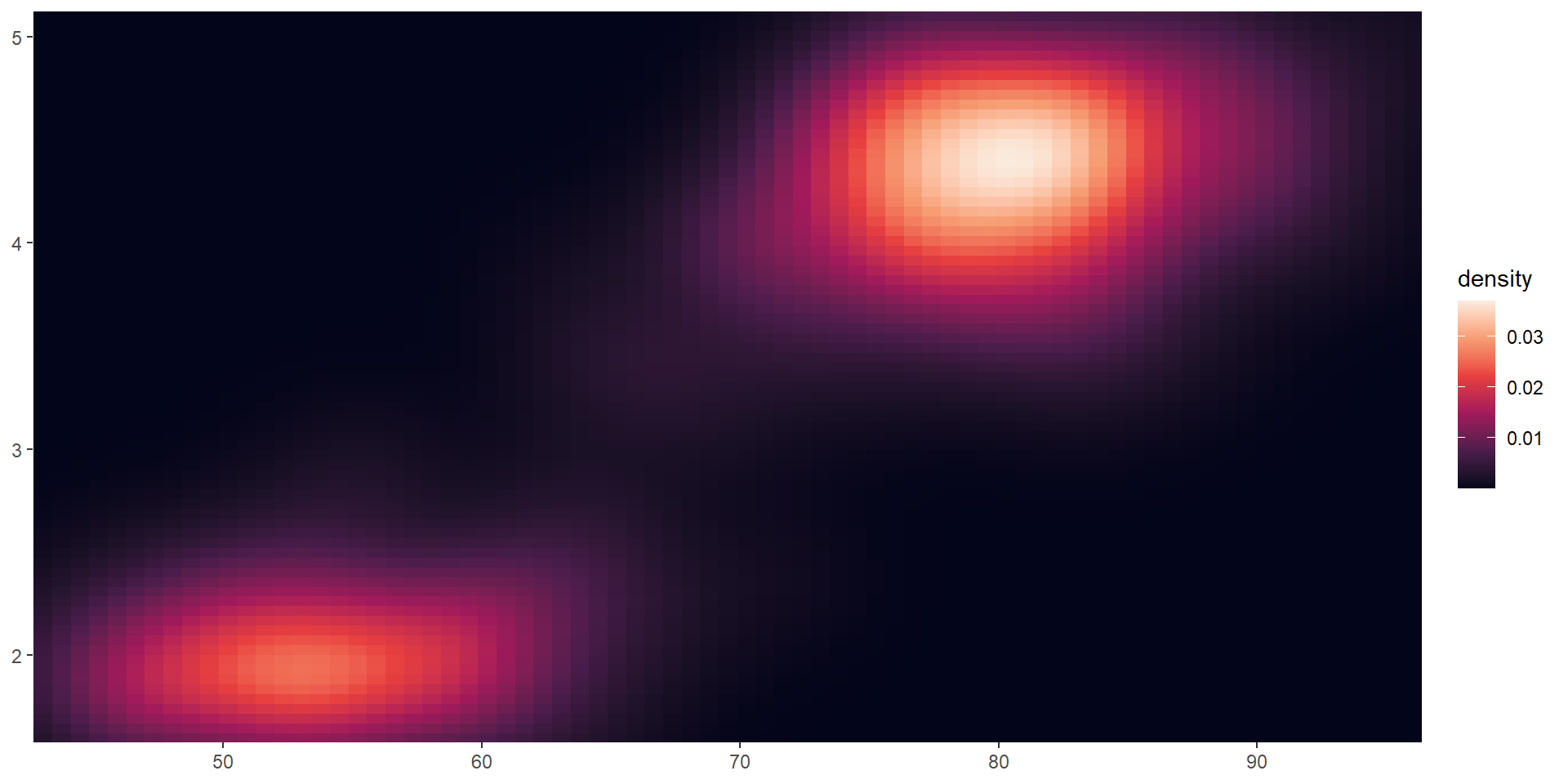
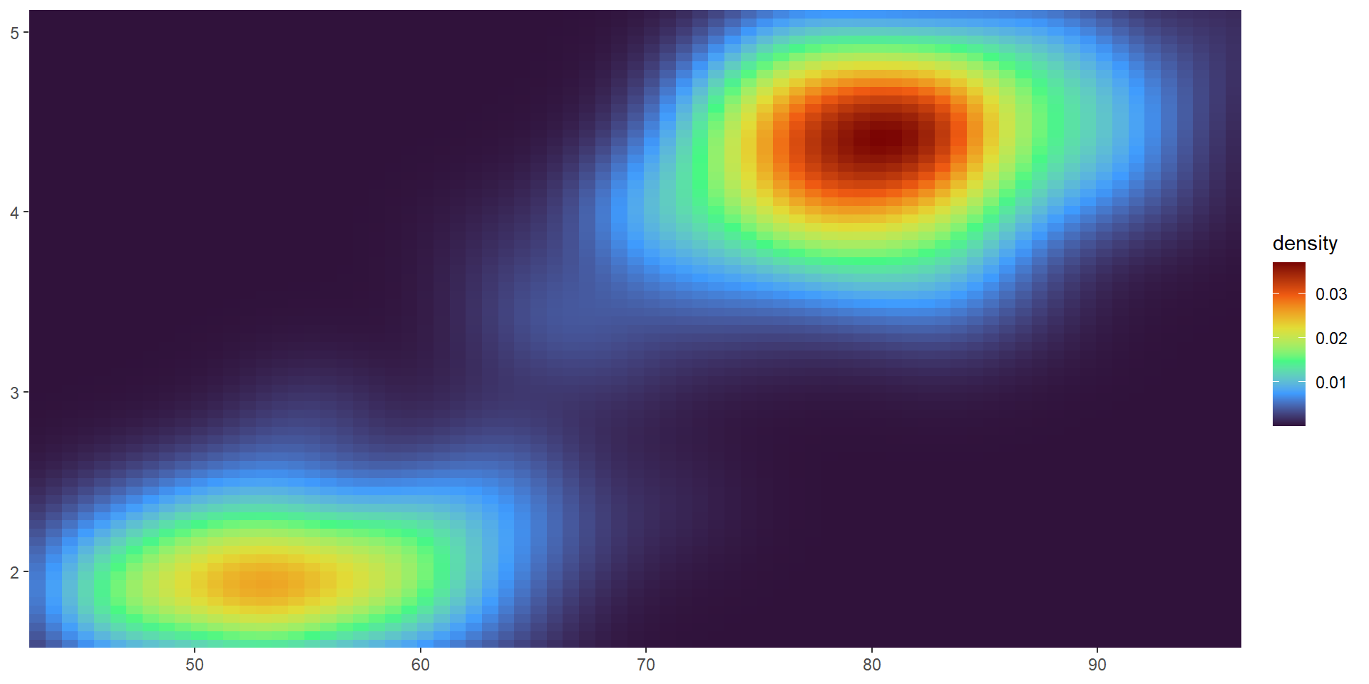
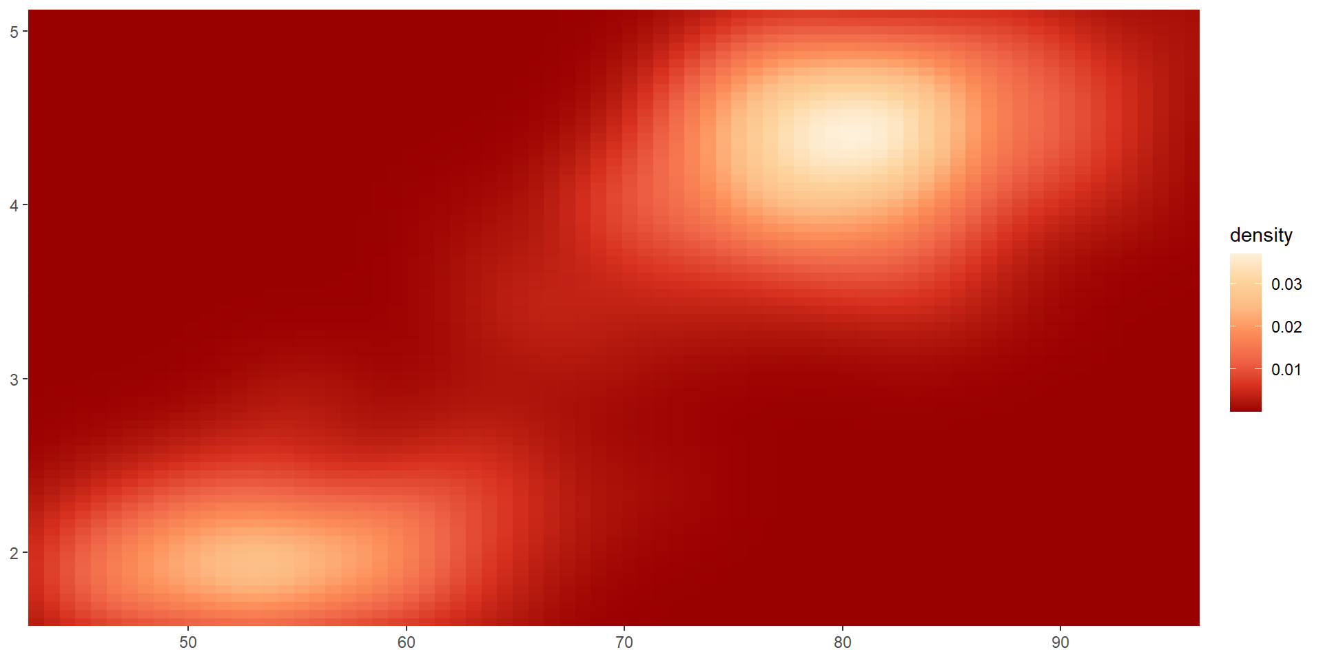
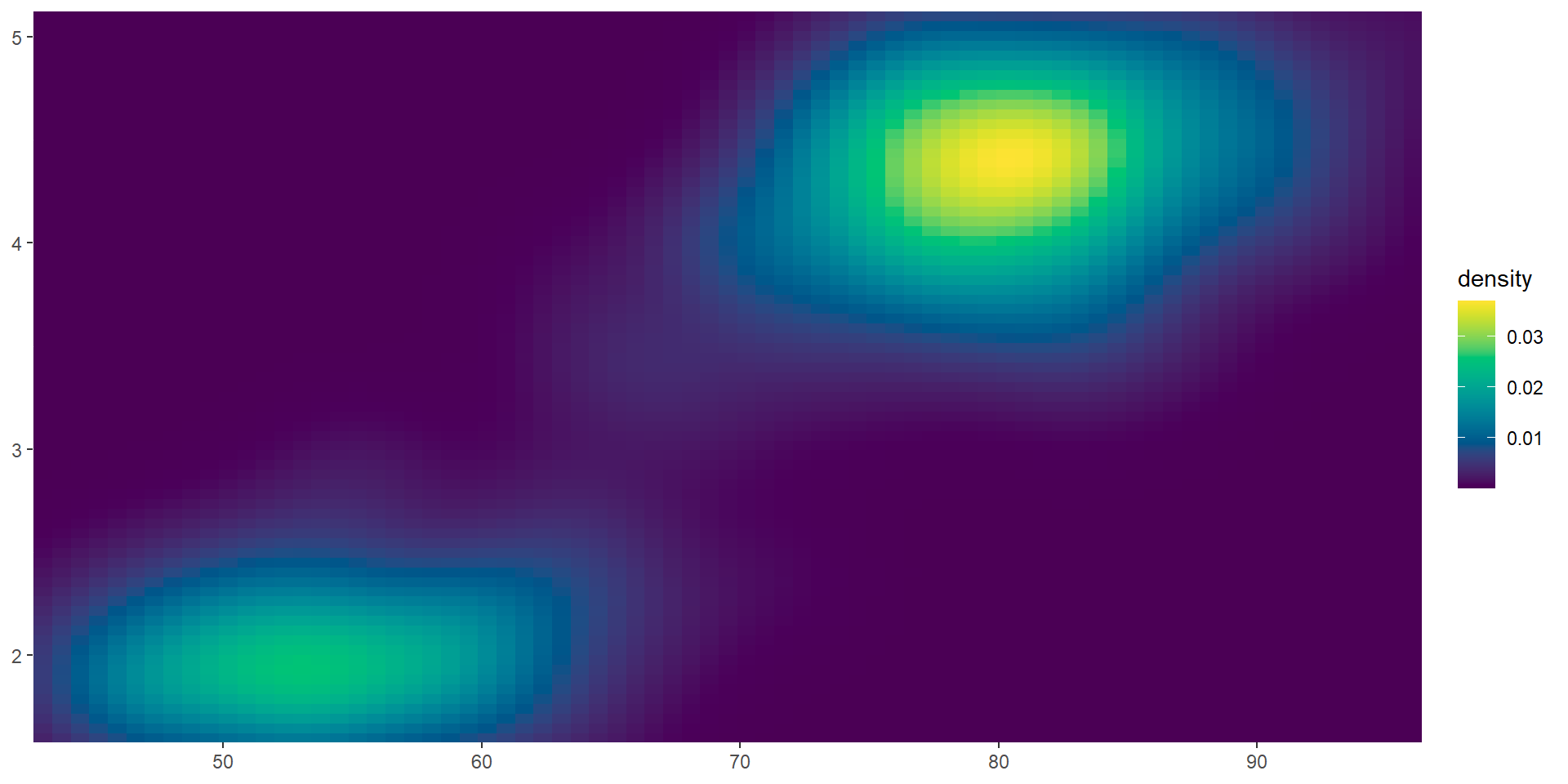
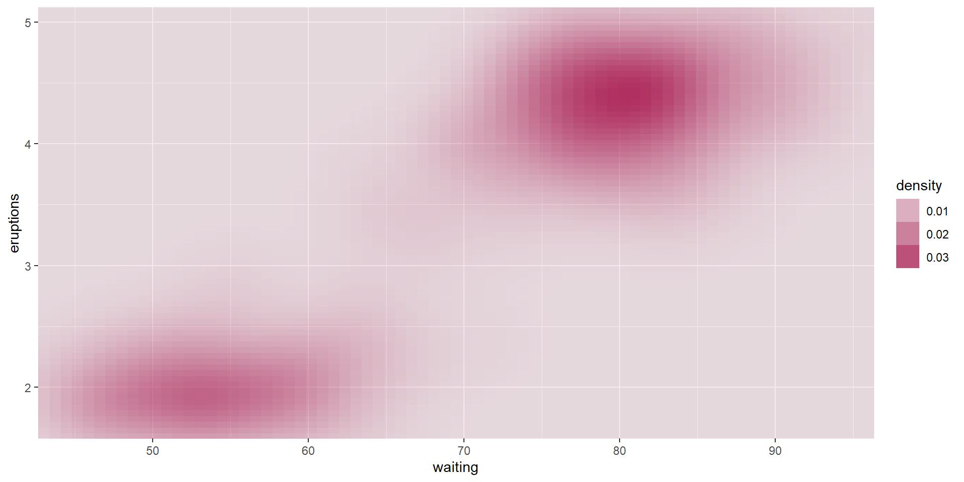
Continuous color scales: viridis color palettes
erupt <- ggplot(faithfuld, aes(waiting, eruptions, fill = density)) +
  geom_raster() + scale_x_continuous(NULL, expand = c(0, 0)) + scale_y_continuous(NULL, expand = c(0, 0))
# Plot
erupt
erupt + scale_fill_viridis_c(option = "viridis")
erupt + scale_fill_viridis_c(option = "magma")
erupt + scale_fill_viridis_c(option = "plasma")
erupt + scale_fill_viridis_c(option = "rocket")
erupt + scale_fill_viridis_c(option = "turbo")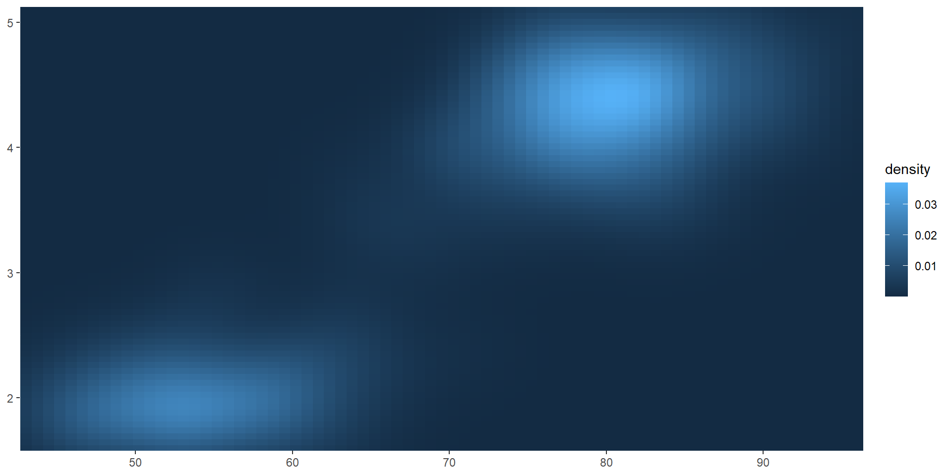
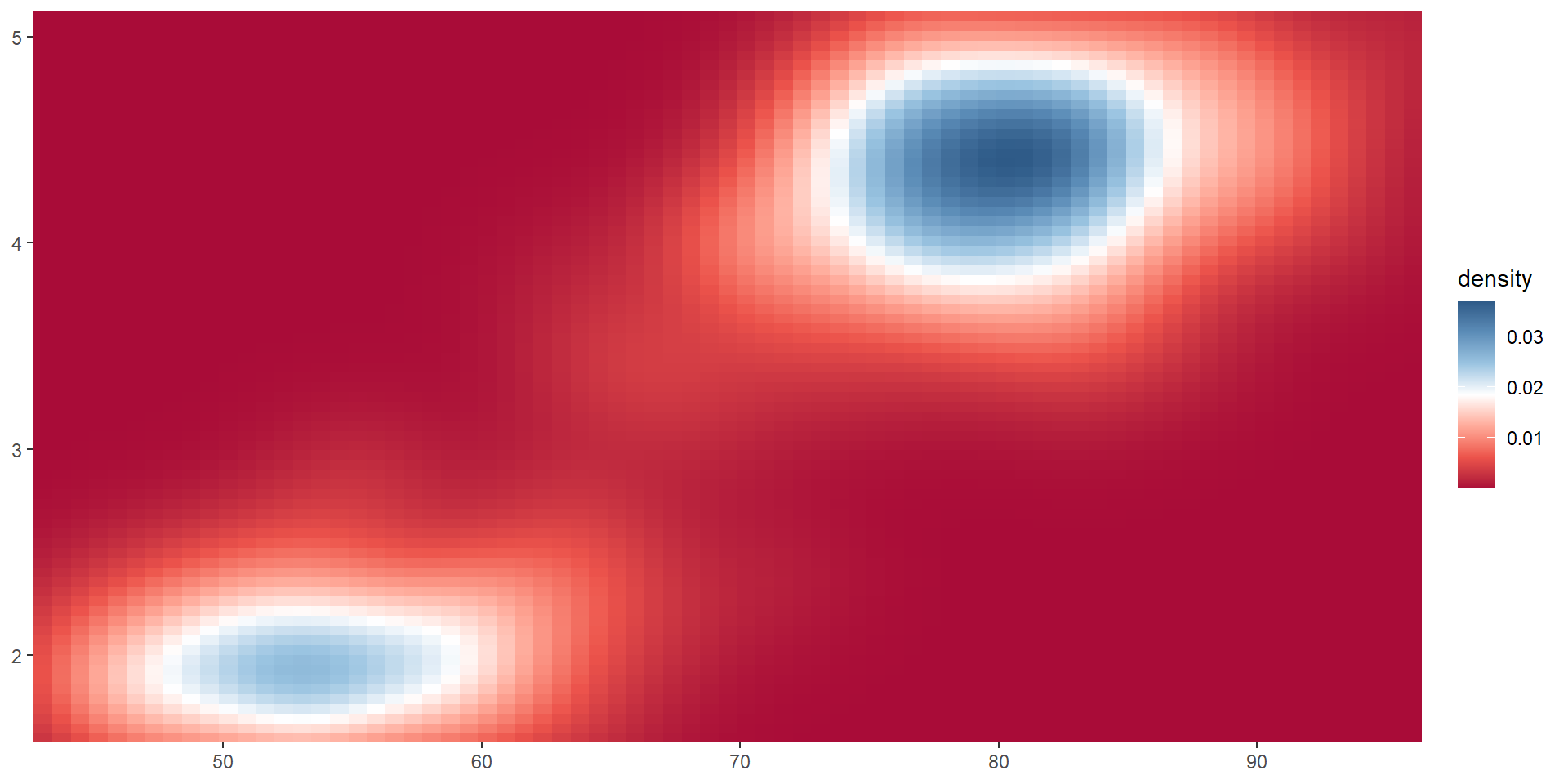
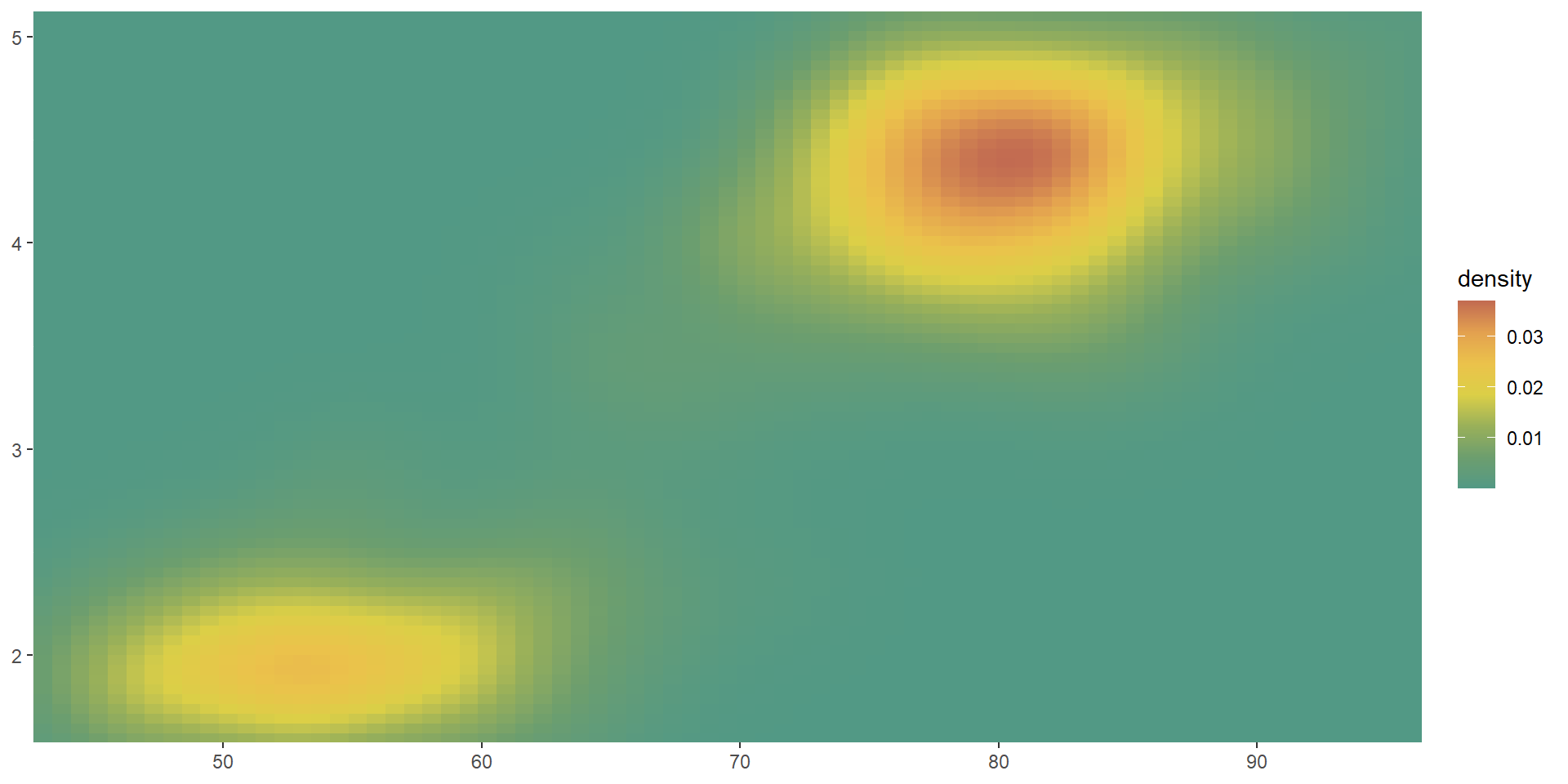
Color scales and legends
Continuous color scales: distiller color palettes
erupt + scale_fill_distiller(palette = "RdBu")
erupt + scale_fill_distiller(palette = "Pastel1")
erupt + scale_fill_distiller(palette = "OrRd")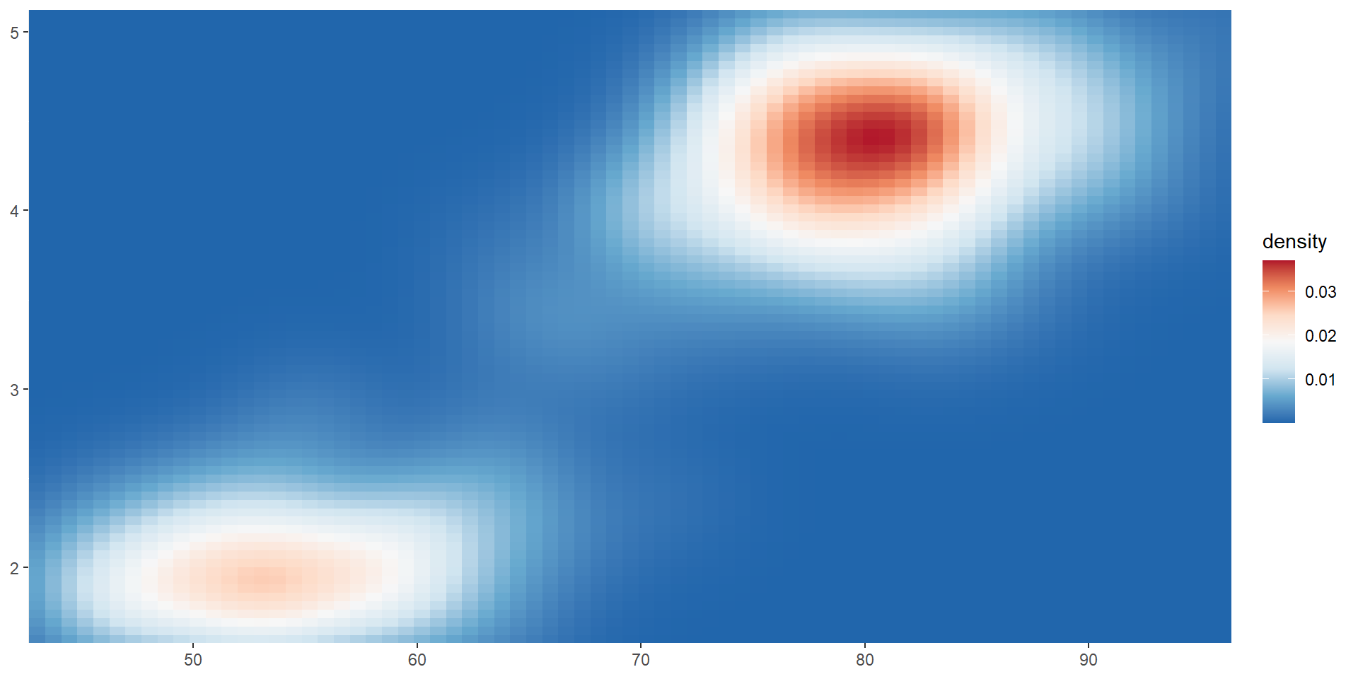
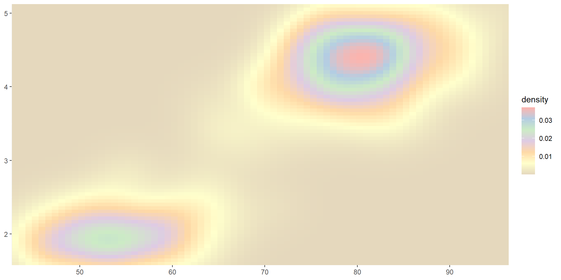
The distiller scales applied brewer color palettes by by smoothly interpolating 7 colors from any palette to a continuous scale. For more brewer color palettes, see https://colorbrewer2.org.
Color scales and legends
Continuous color scales: ggsci color palettes
library(ggsci)
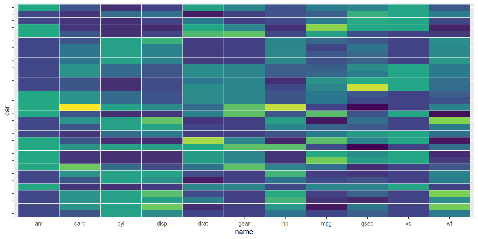
dt_hm <- scale(as.matrix(mtcars)[1:10, ], center = TRUE, scale = TRUE)
p_hm <- as.data.frame(dt_hm) %>% rownames_to_column(var = "cars") %>%
pivot_longer(!cars) %>%
ggplot(aes(x = name, y = cars, fill = value)) +
geom_tile(color = "black") +
coord_equal() +
labs(x=NULL, y = NULL) +
theme(legend.position = "none",
axis.text.x = element_blank())
p_hm
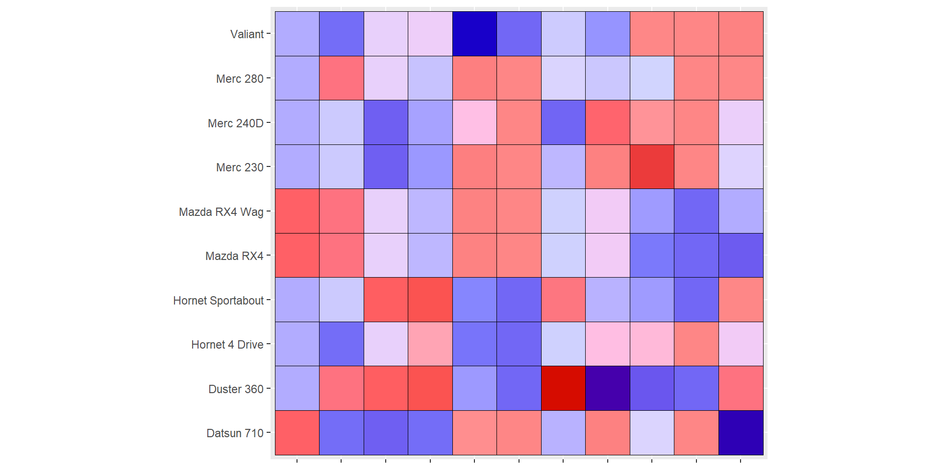
p_hm + scale_fill_gsea()
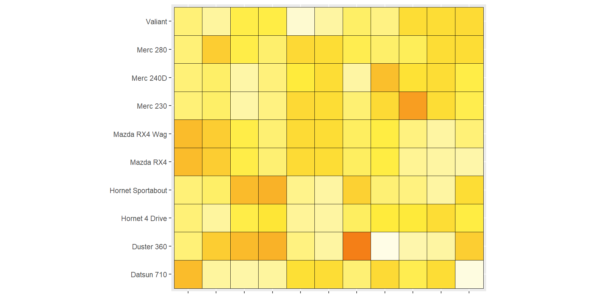
p_hm + scale_fill_material("yellow")
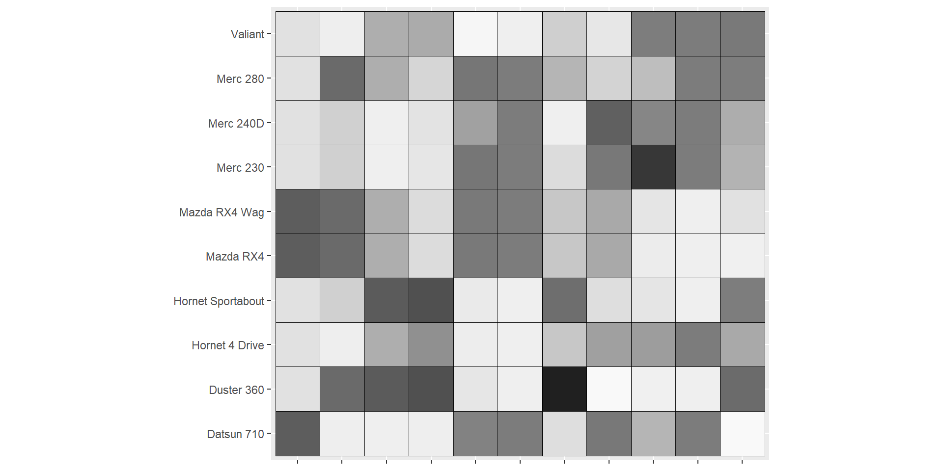
p_hm + scale_fill_material("grey")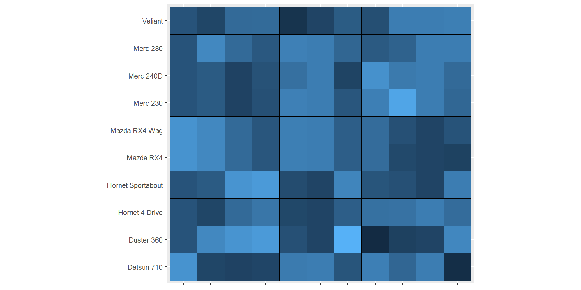
Discover more continuous ggsci color palette: https://cran.r-project.org/web/packages/ggsci/vignettes/ggsci.html
Color scales and legends
More Continuous color scales: paletteer color palettes
erupt + scale_fill_paletteer_c("ggthemes::Green-Blue Diverging")
erupt + scale_fill_paletteer_c("ggthemes::Red-Blue-White Diverging")
erupt + scale_fill_paletteer_c("ggthemes::Temperature Diverging")
erupt + scale_fill_paletteer_c("grDevices::rainbow")
erupt + scale_fill_paletteer_c("grDevices::heat.colors")
erupt + scale_fill_paletteer_c("grDevices::Viridis")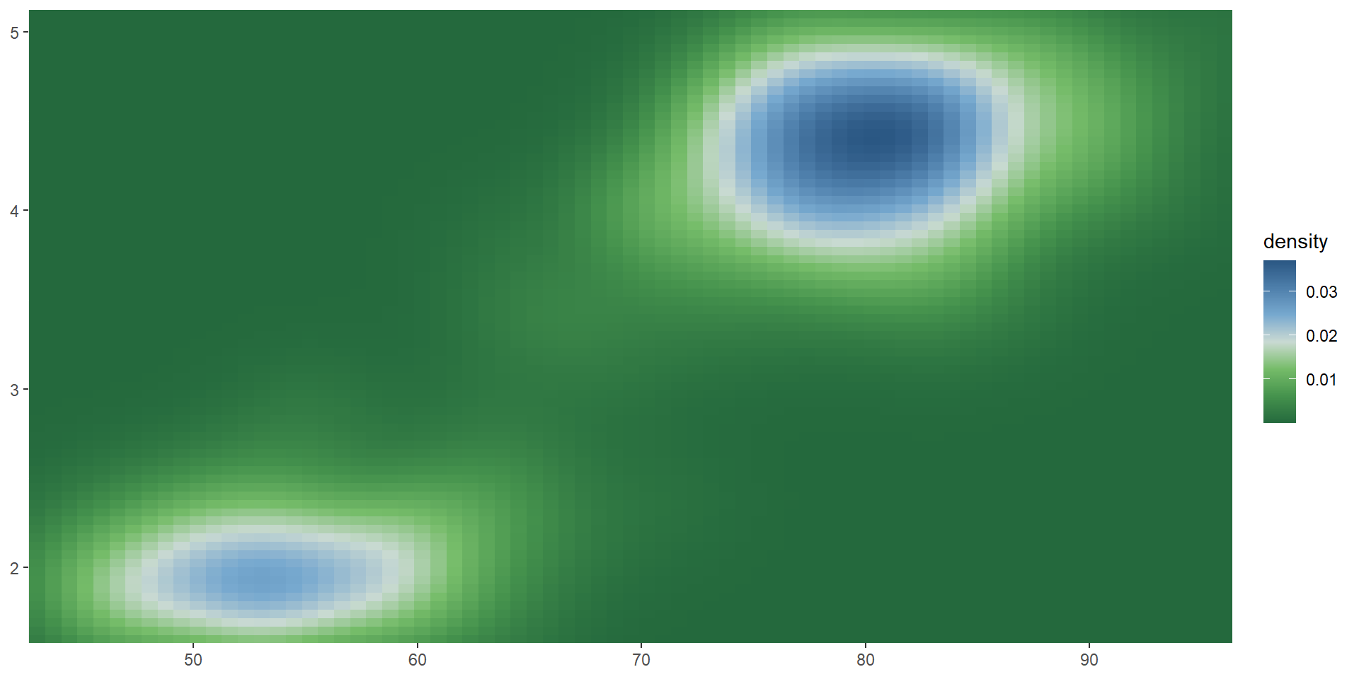
More continuous paletteer color palettes can be found at: https://pmassicotte.github.io/paletteer_gallery.
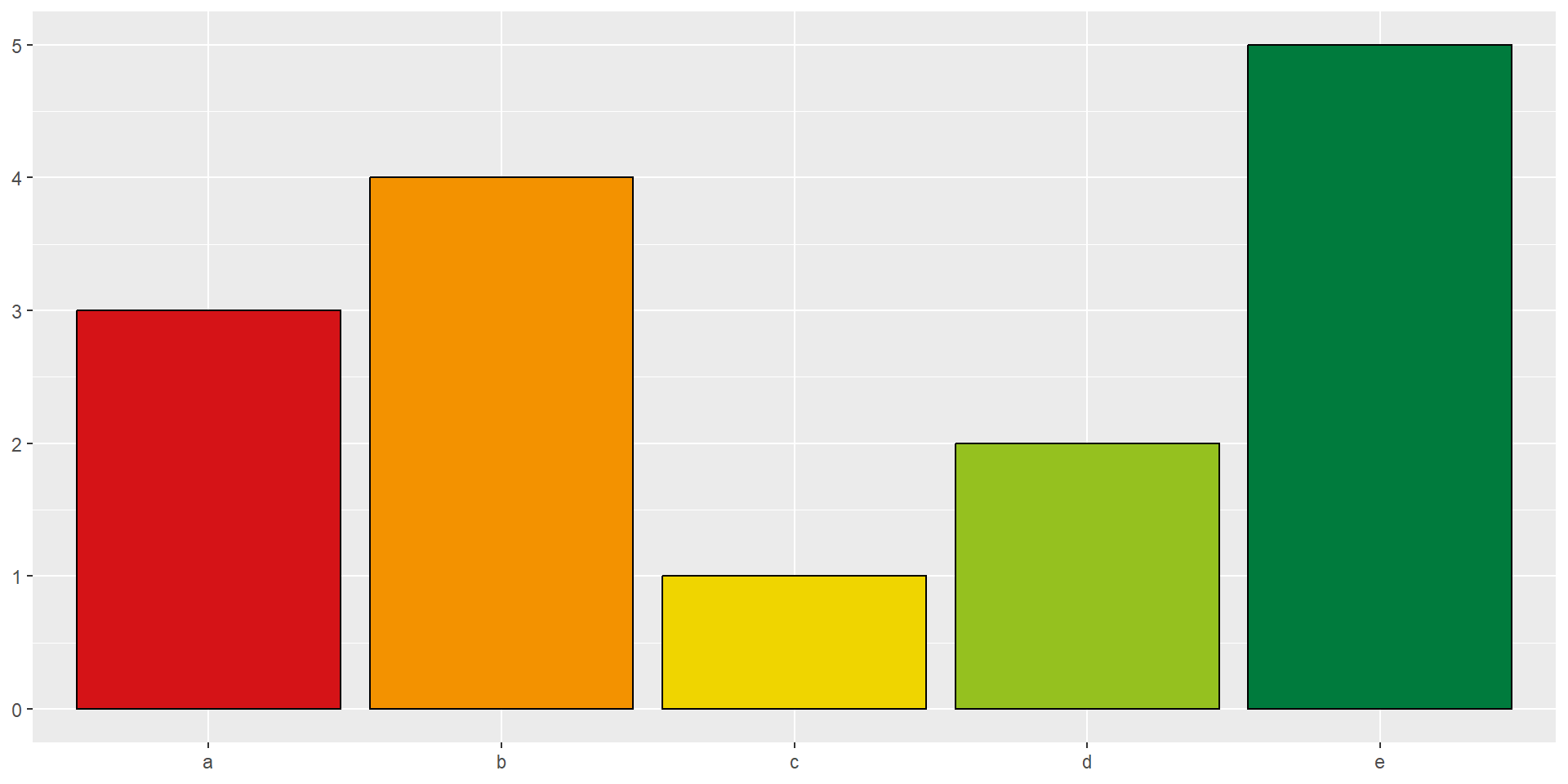
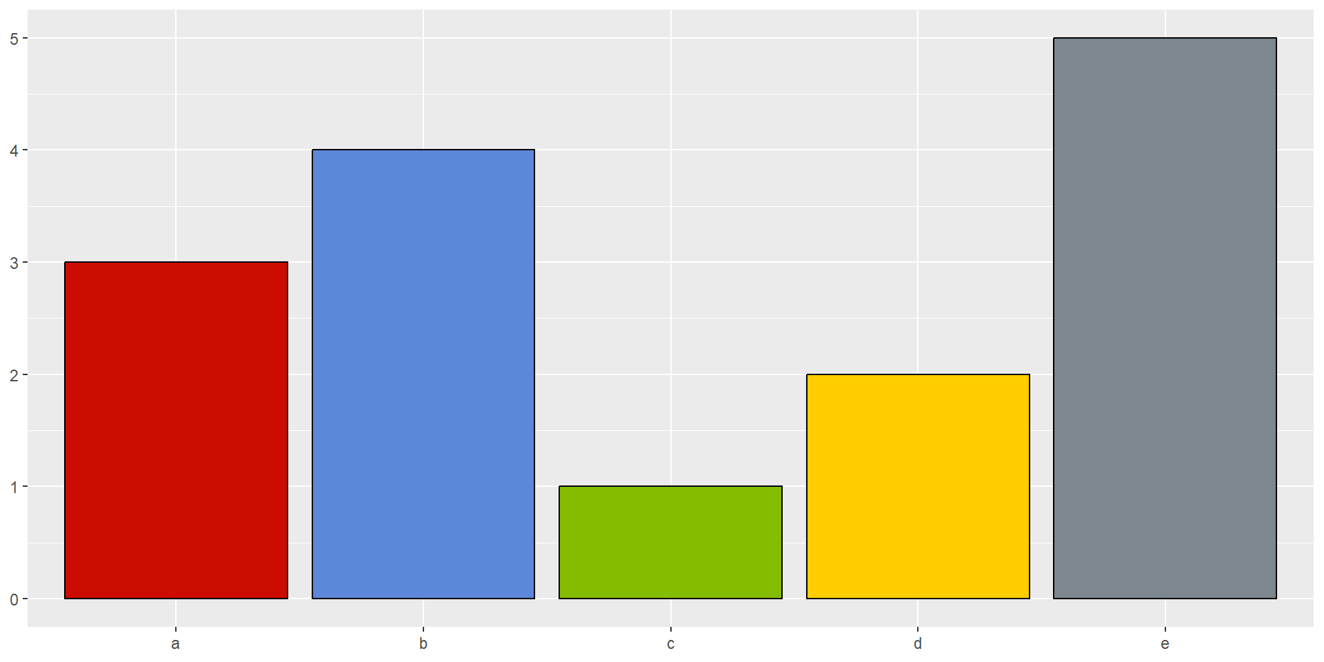
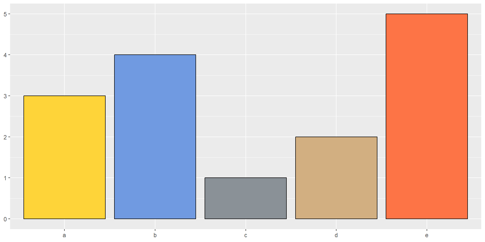
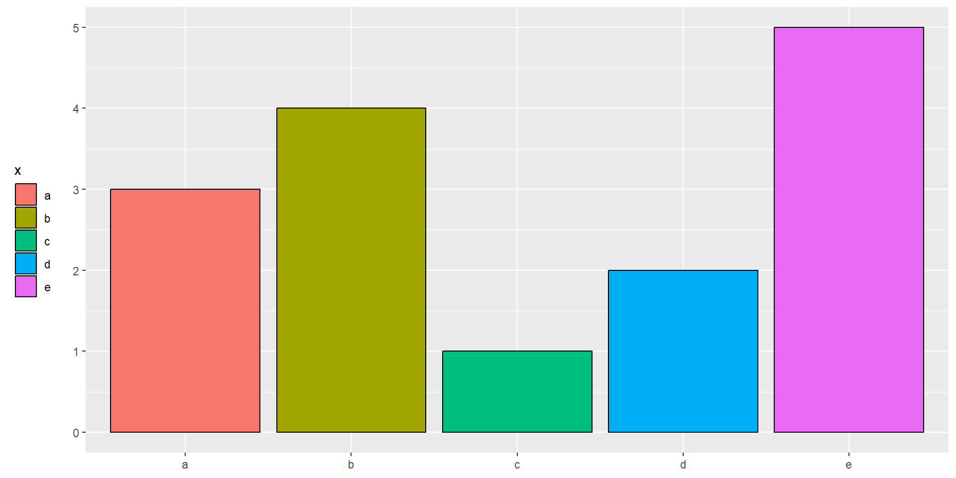
Color scales and legends
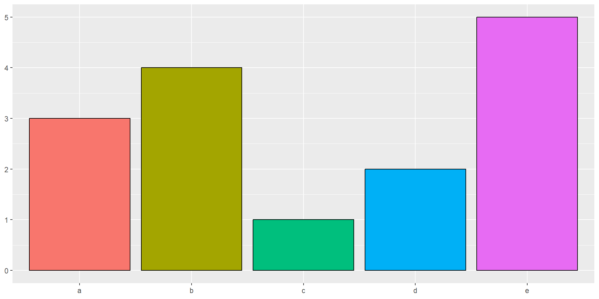
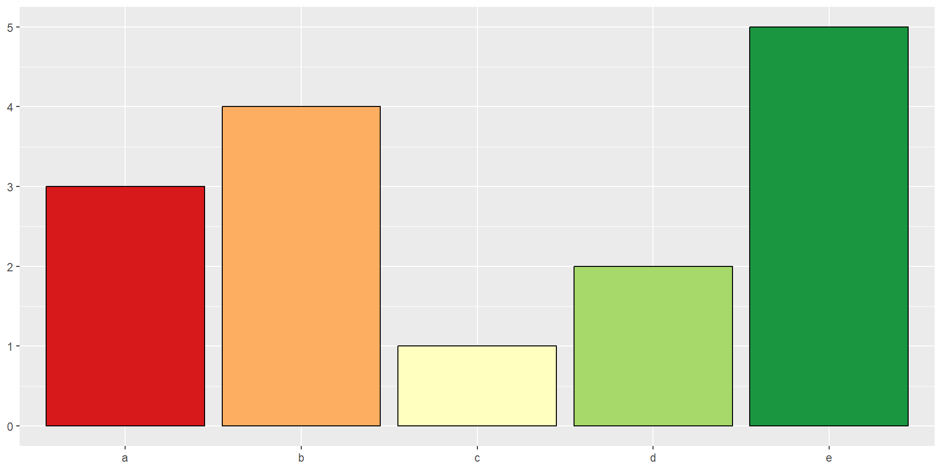
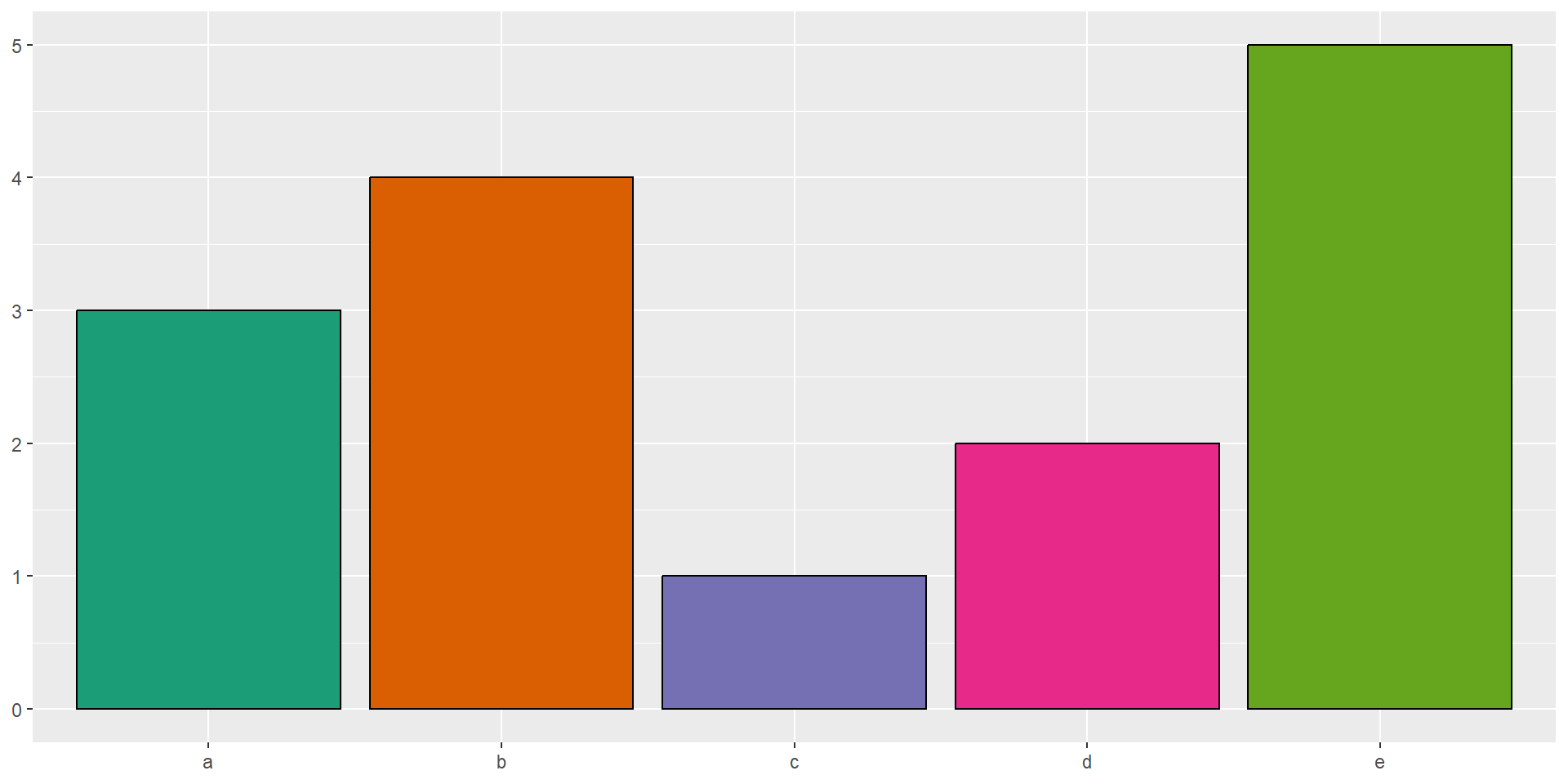
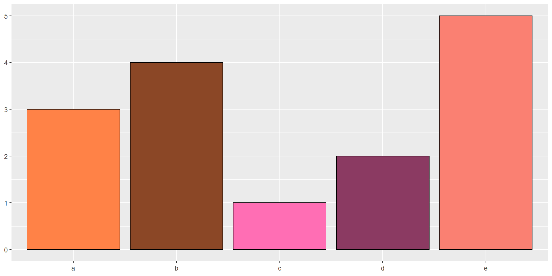
Discrete color scales: default palette

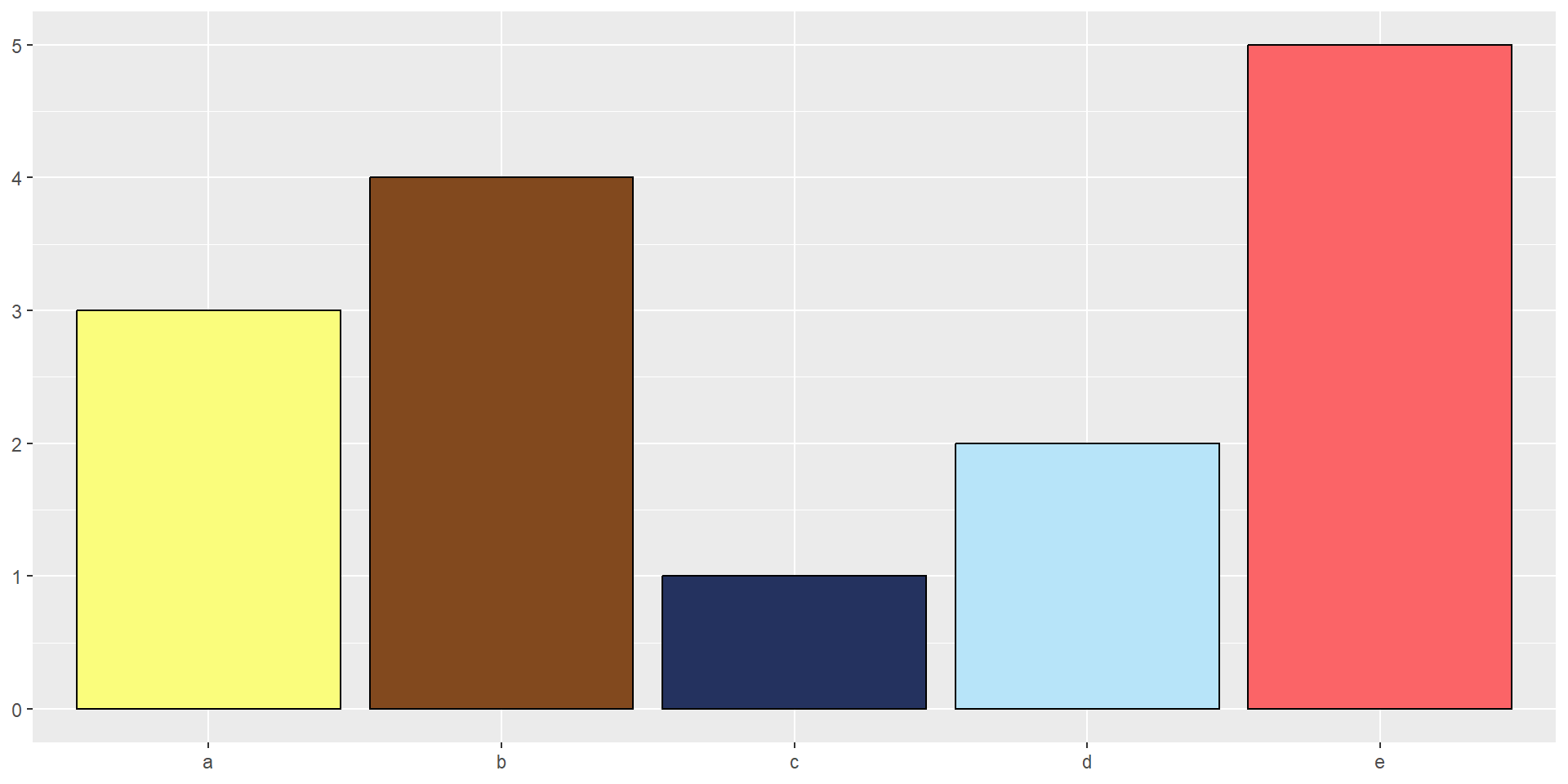
Color scales and legends
Discrete color scales: RColorBrewer palettes
bars + scale_fill_brewer(palette = "BrBG")
bars + scale_fill_brewer(palette = "RdYlGn")
bars + scale_fill_brewer(palette = "Dark2")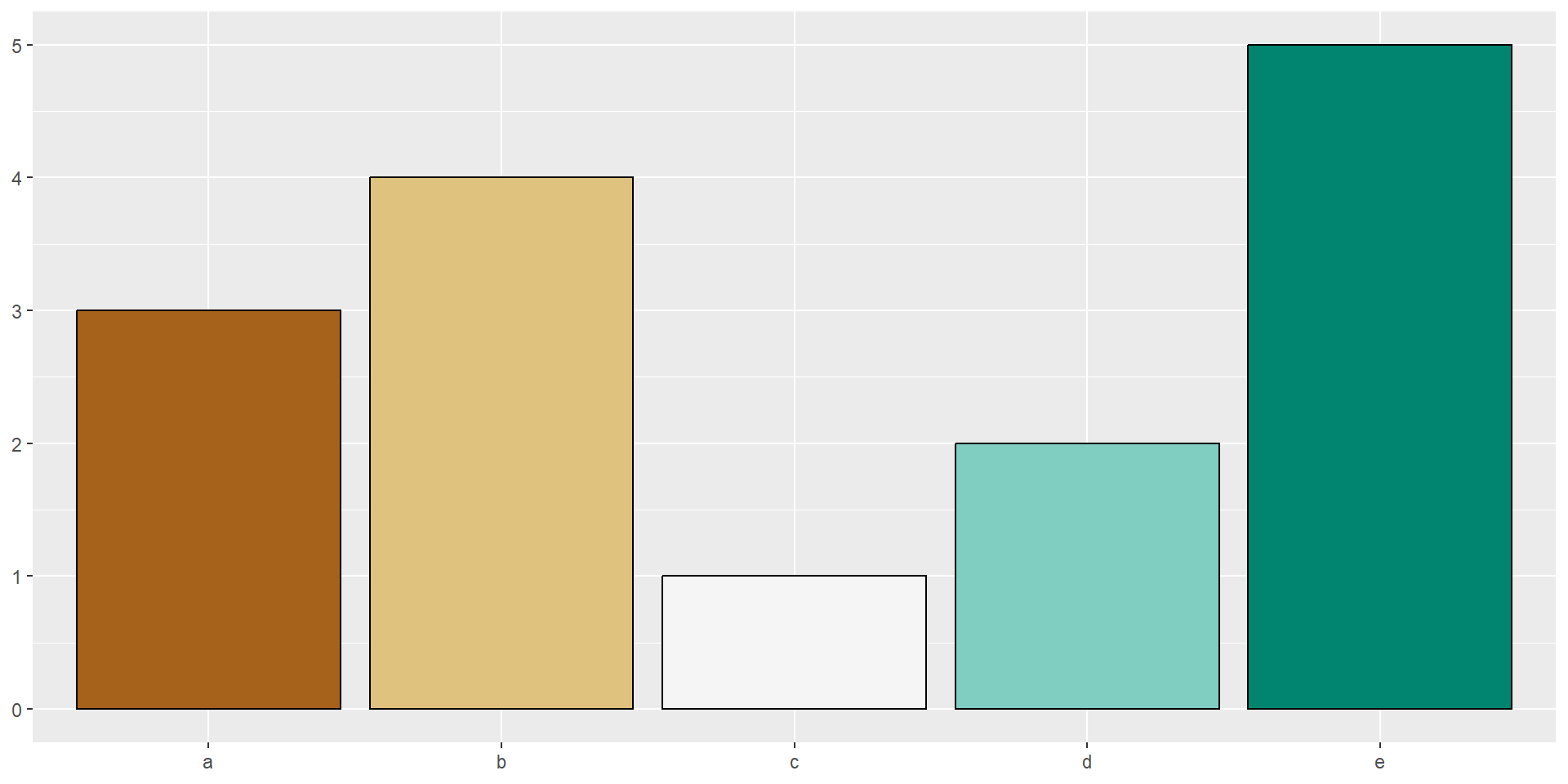
Interactive RColorBrewer picker: https://colorbrewer2.org
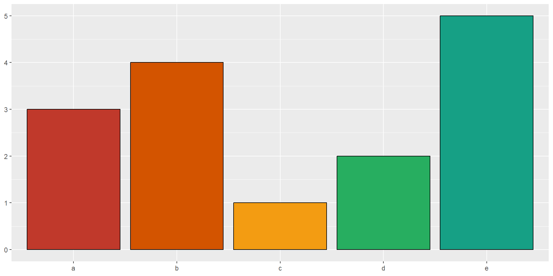
Color scales and legends
Discrete color scales: ggsci palettes
ggsci offers high-quality color palettes based on color schemes used in scientific journals, data visualization libraries, and science fiction movies.
bars + scale_fill_aaas()
bars + scale_fill_npg()
bars + scale_fill_nejm()
bars + scale_fill_frontiers()
bars + scale_fill_rickandmorty()
bars + scale_fill_flatui()
bars + scale_fill_startrek()
bars + scale_fill_simpsons()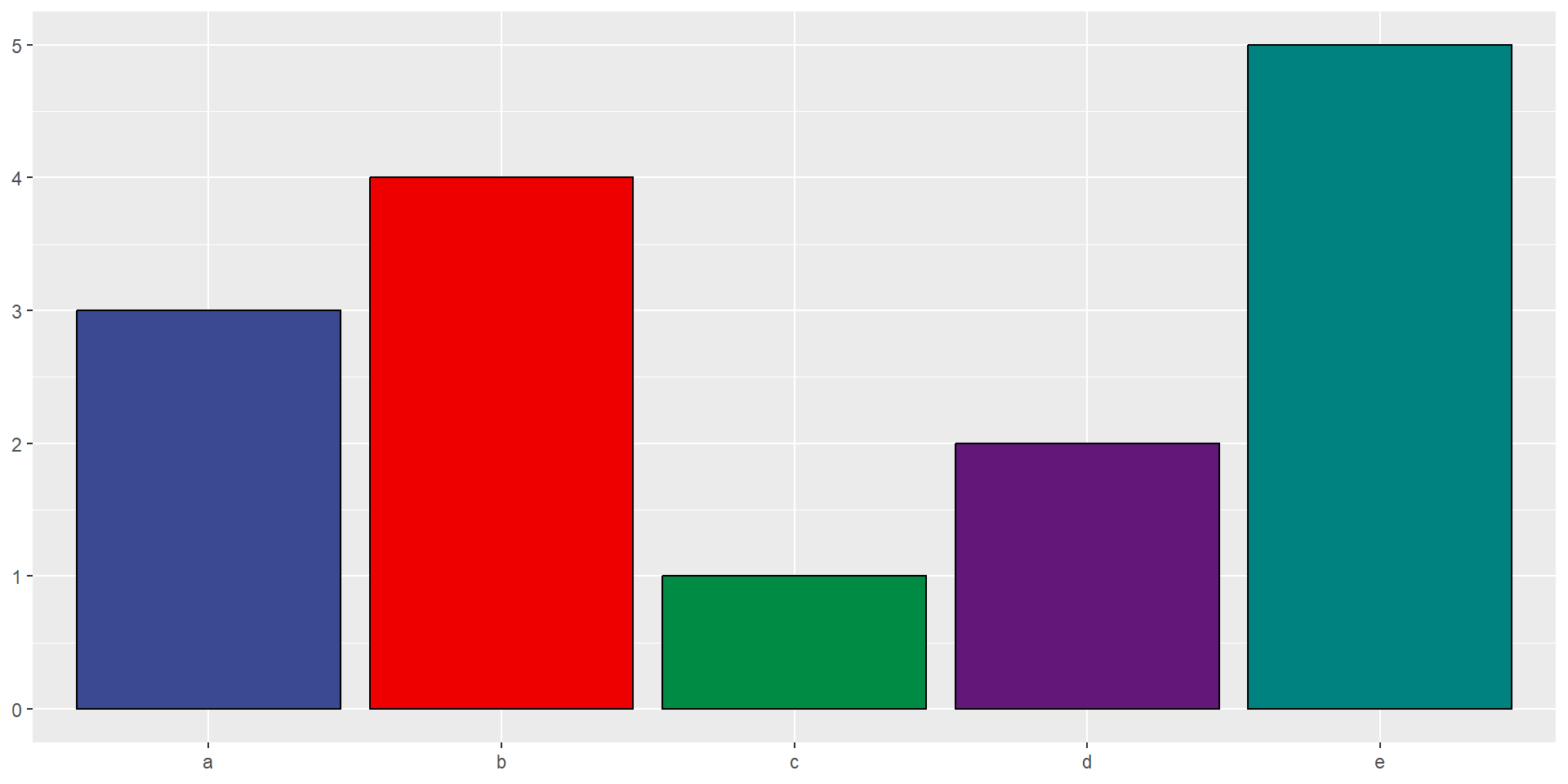
Color scales and legends
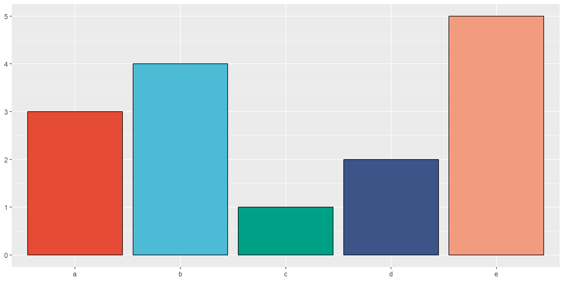
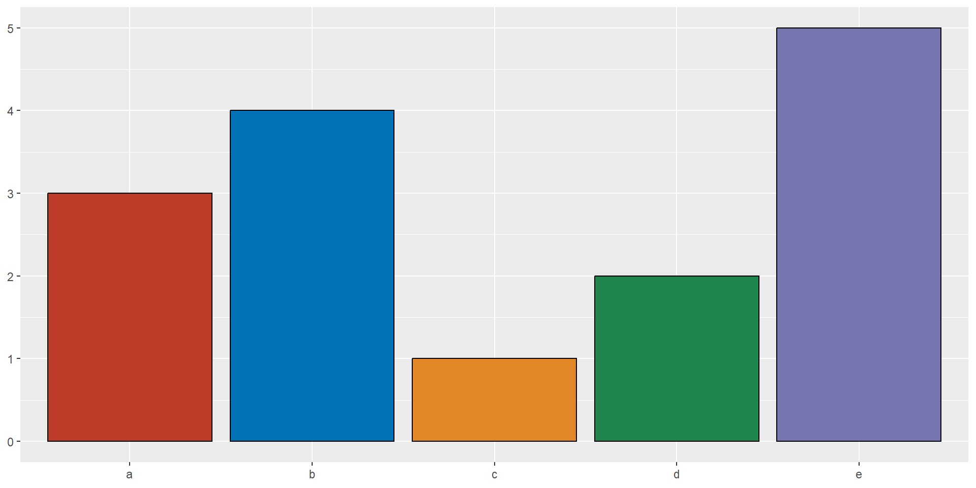
More discrete color scales from paletteer
bars + scale_fill_paletteer_d("awtools::bpalette")
bars + scale_fill_paletteer_d("basetheme::ink")
bars + scale_fill_paletteer_d("calecopal::kelp1")
bars + scale_fill_paletteer_d("fishualize::Centropyge_loricula")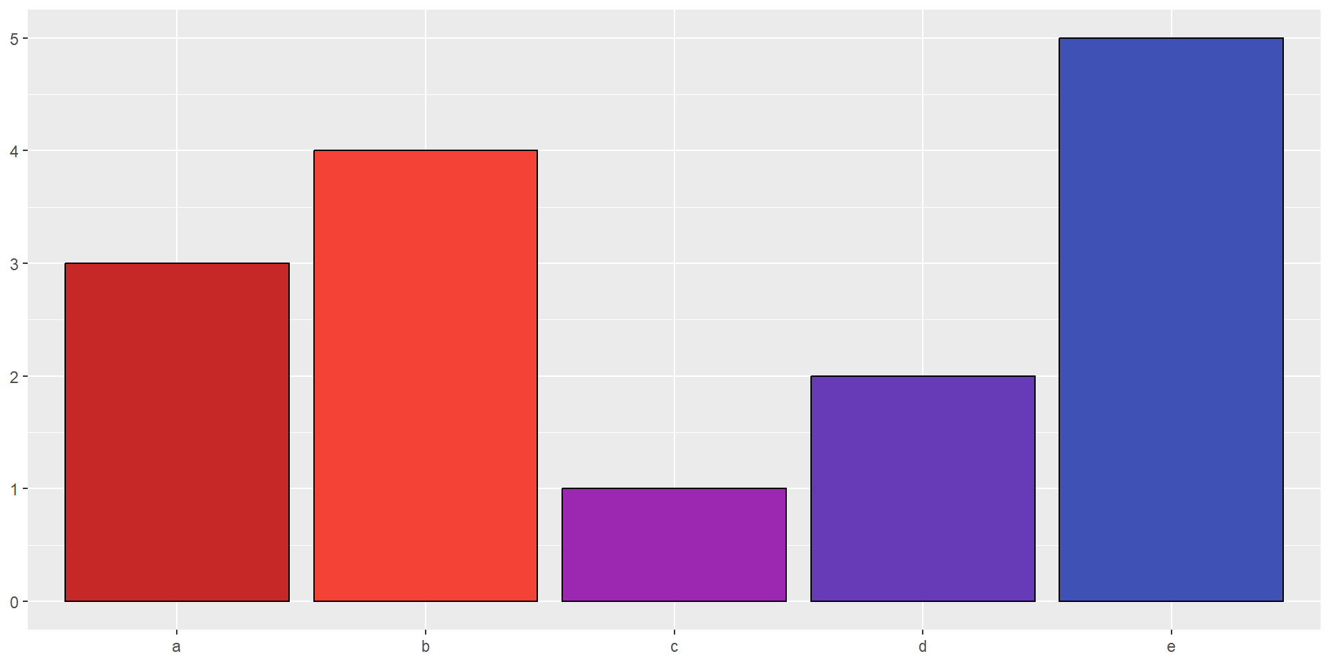
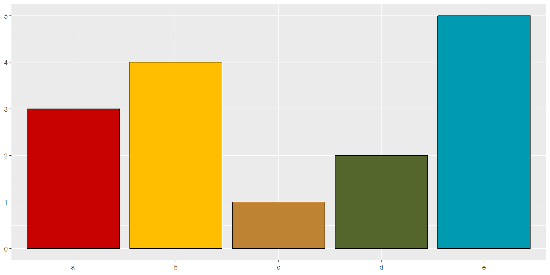

Interactive discrete paletteer color palette: https://emilhvitfeldt.github.io/r-color-palettes/discrete.html
Color scales and legends
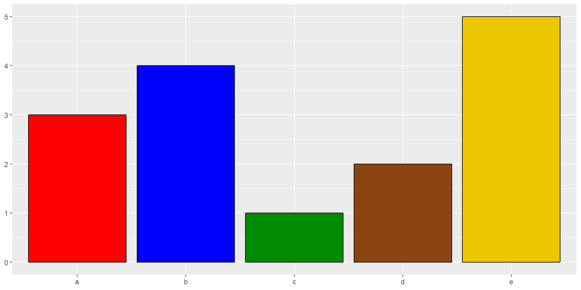
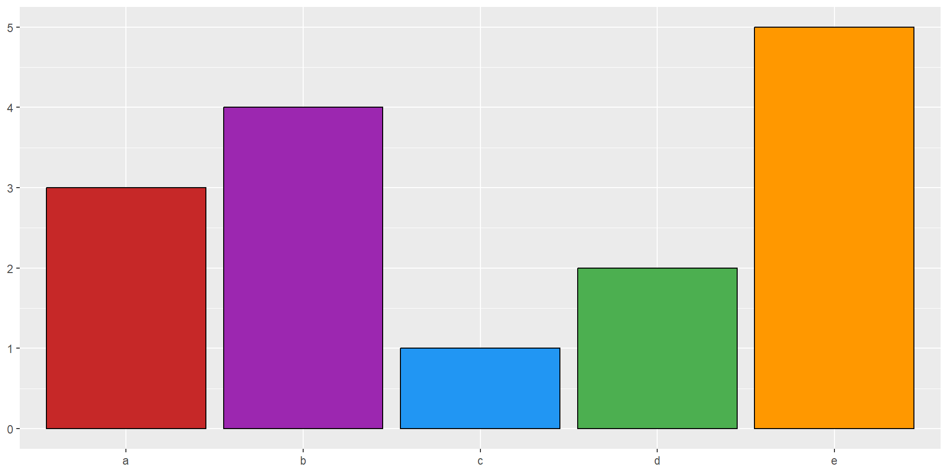
Manual discrete color scale
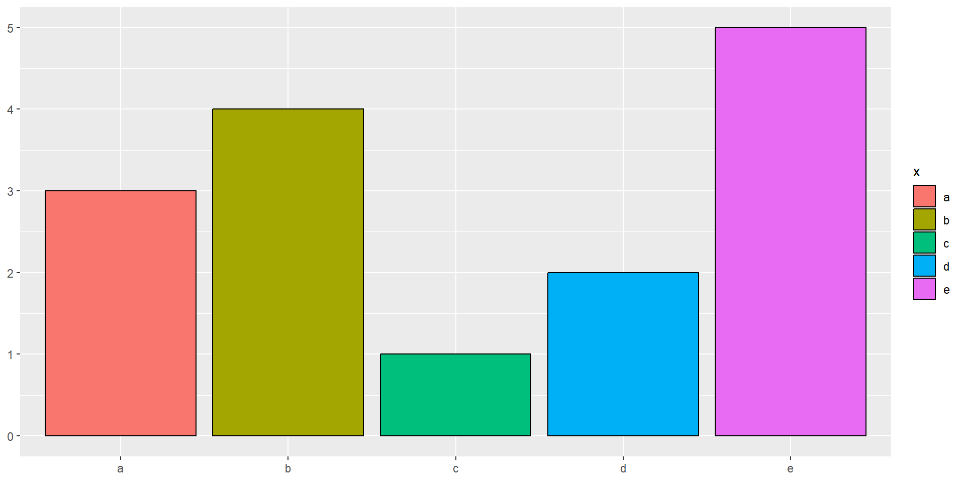
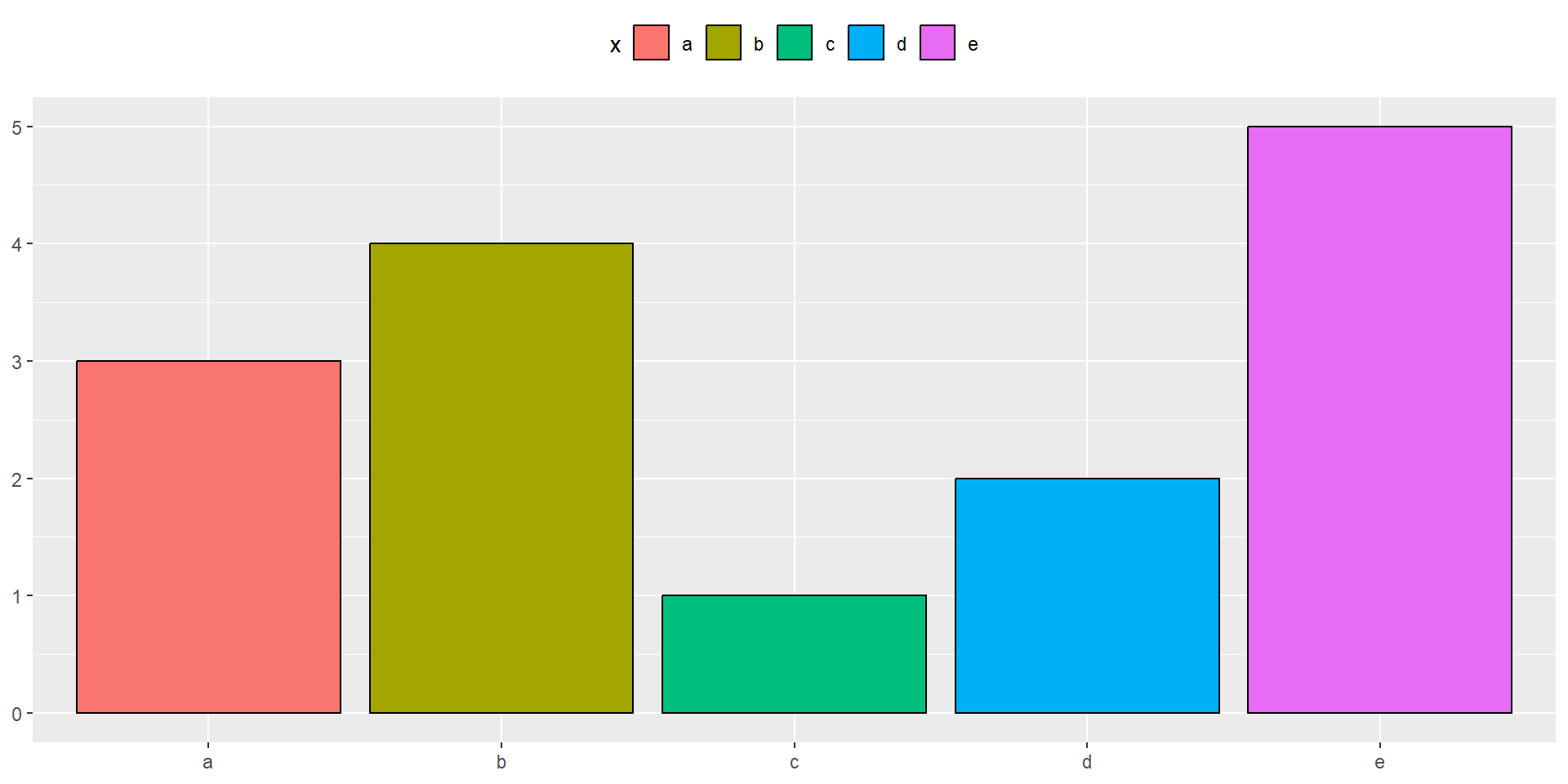
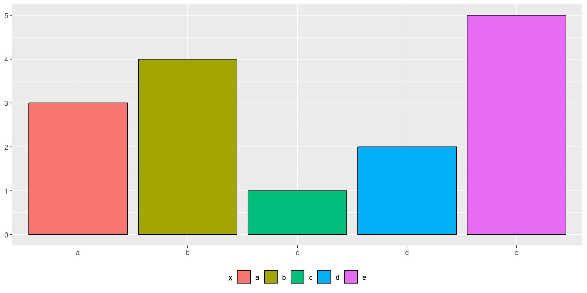
Color scales and legends
Alpha
The alpha scale maps shade transparency to a numerical value.
Color scales and legends
Legend positions

References
ggplot2: Elegant Graphics for Data Analysis (3e): written by Hadley Wickham, Danielle Navarro, and Thomas Lin Pedersen (2023).
Introduction to data visualisation with ggplot2 Workshop: by QCBS R Workshop Series, 2023-04-24
Fundamentals of Data Visualization: by Claus O. Wilke, 2019