| Name | Length | EffectiveLength | TPM | NumReads |
|---|---|---|---|---|
| TRINITY_DN35101_c0_g1 | 248 | 35.30 | 0.00 | 0.00 |
| TRINITY_DN42970_c0_g1 | 215 | 24.82 | 7.15 | 3.00 |
| TRINITY_DN41199_c0_g1 | 280 | 47.38 | 0.00 | 0.00 |
| TRINITY_DN35784_c0_g1 | 247 | 34.96 | 6.77 | 4.00 |
| TRINITY_DN32682_c0_g1 | 275 | 45.30 | 0.00 | 0.00 |
| TRINITY_DN8538_c0_g1 | 1019 | 710.33 | 0.17 | 2.00 |
| TRINITY_DN2880_c0_g1 | 2376 | 2067.33 | 0.74 | 26.00 |
| TRINITY_DN9226_c0_g1 | 275 | 45.30 | 7.84 | 6.00 |
| TRINITY_DN3645_c1_g1 | 1175 | 866.33 | 0.40 | 5.82 |
| TRINITY_DN5921_c0_g2 | 368 | 94.72 | 4.37 | 7.00 |
6 Estimating Abundance and Differential Expression Analysis of Genes
Differential gene expression analysis is a statistical method that uses count data to determine significant changes between experimental groups. For example, transcriptional changes of stress-induced genes in plant leaves under water deficit compared to normal conditions are examined. Count data can be transcript, gene, exon, and noncoding characteristics.
To perform differential gene expression analysis with the Trinity integrated extensions, you will need the assembled transcripts/genes from the previous step and clean reads (and their replicates) from your experiment to assign to the assembled transcripts/genes and count the number of reads assigned to those transcripts/genes.
6.1 Estimating Transcript Abundance
This part will adopted from Trinity’s Wiki Trinity Transcript Quantification.
There are two different methods for quantifying reads mapped to the reference, by using the alignment-based (RSEM) and alignment-free (salmon, kallisto) qualtifiers. In this workshop, we’ll use the salmon, an ultra-fast alignment and quantification tool, to count number of reads mapped to the assembled gene.
Tip
You can see the usage of the command you wsh to perform by type the command followed by --help, or -h. For example, to see the usage of
align_and_estimate_abundance.pl -h
Activity
Now we will align and count reads mapped to the reference assembled transcripts using buit-in utility align_and_estimate_abundance.pl using the following commands.
- Go to working directory and activate conda environment
Go to working directory
cd ~/Cpa_RNASeqThe working directory should contain the following subdirectories.
Cpa_RNASeq
    ├── 01_Rawdata
    ├── 02_QC
    ├── 03_assembly
    ├── 04_DE_analysis
    └── 05_annotation
Then, activate conda environment
conda activate trinity- Estimating Transcript Abundance
your current working directory is: ~/Cpa_RNASeq
align_and_estimate_abundance.pl \
--transcripts 03_assembly/Trinity_2023-03-08.Trinity.fasta \
--seqType fq \
--samples_file /opt/Cpa_RNASeq/sample_list.tsv \
--est_method salmon \
--gene_trans_map 03_assembly/Trinity_2023-03-08.Trinity.fasta.gene_trans_map \
--thread_count 2 \
--prep_reference
Then, type ls to see the results in your working directory. These directories are the results from the above command. Each folder represents each biological replicate in your experiment.
drwxrwxr-x  5 jiratchaya jiratchaya 4096 Mar  9 20:37 dark_1/
drwxrwxr-x  5 jiratchaya jiratchaya 4096 Mar  9 20:38 dark_2/
drwxrwxr-x  5 jiratchaya jiratchaya 4096 Mar  9 20:38 dark_3/
drwxrwxr-x  5 jiratchaya jiratchaya 4096 Mar  9 20:38 normal_light_1/
drwxrwxr-x  5 jiratchaya jiratchaya 4096 Mar  9 20:39 normal_light_2/
drwxrwxr-x  5 jiratchaya jiratchaya 4096 Mar  9 20:39 normal_light_3
Estimated time usage: ~ 20 min per user
Parameter descriptions of align_and_estimate_abundance.pl: the assembled transcripts flagged in --transcripts, --seqType indicates file format of reads that will be mappped to the reference transcripts. We define the read count estimation tool in --est_method, in this workshop we use salmon, and also estimate read counts using information of gene-transcript relationships from the trinity_out_dir.Trinity.fasta.gene_trans_map file that we specified in the --gene_trans_map parameter.
A list of read files will be contained in the metadata file sample_list.tsv in the parameter --samples_file, which we have prepared for you. In short, the sample list will be prepared in a tab-delimited text file indicating the relationships between biological replicates. For example,
jiratchaya@pslab1:~$ cat /opt/Cpa_RNASeq/sample_list.tsv
dark    dark_1  /opt/Cpa_RNASeq/Cyanophora_rawdata/SRR8306034_1.fastq   /opt/Cpa_RNASeq/Cyanophora_rawdata/SRR8306034_2.fastq
dark    dark_2  /opt/Cpa_RNASeq/Cyanophora_rawdata/SRR8306029_1.fastq   /opt/Cpa_RNASeq/Cyanophora_rawdata/SRR8306029_2.fastq
dark    dark_3  /opt/Cpa_RNASeq/Cyanophora_rawdata/SRR8306028_1.fastq   /opt/Cpa_RNASeq/Cyanophora_rawdata/SRR8306028_2.fastq
normal_light    normal_light_1  /opt/Cpa_RNASeq/Cyanophora_rawdata/SRR8306033_1.fastq   /opt/Cpa_RNASeq/Cyanophora_rawdata/SRR8306033_2.fastq
normal_light    normal_light_2  /opt/Cpa_RNASeq/Cyanophora_rawdata/SRR8306032_1.fastq   /opt/Cpa_RNASeq/Cyanophora_rawdata/SRR8306032_2.fastq
normal_light    normal_light_3  /opt/Cpa_RNASeq/Cyanophora_rawdata/SRR8306035_1.fastq   /opt/Cpa_RNASeq/Cyanophora_rawdata/SRR8306035_2.fastq
The first column indicates the study experimental groups, followed by their biological replicates in the second column, and the forward and reverse sequence read files belong to their biological replicate. It’s important that the file path begins with the directory in which you’ll be working so that the programs can correctly route to the files.
Output results are created in the current working directory separately for experimental groups and biological replicates as follow.
dark_1
    ├── aux_info/
    ├── cmd_info.json
    ├── lib_format_counts.json
    ├── libParams/
    ├── logs/
    ├── quant.sf
    └── quant.sf.genes
.
.
.
normal_light_3
    ├── aux_info/
    ├── cmd_info.json
    ├── lib_format_counts.json
    ├── libParams/
    ├── logs/
    ├── quant.sf
    └── quant.sf.genes
Activity
According to the previous part, now we’ll organize the directory to make it tidy by moving all the results to the directory 04_DE_analysis.
# make sure you're in ~/Cpa_RNASeq directory so that you can move the file correctly.
mv dark* normal* 04_DE_analysis/

# Then enter to the directory `04_DE_analysis`
cd 04_DE_analysis
ls ./*
Expected result:
(trinity) jiratchaya@pslab1:~/Cpa_RNASeq/04_DE_analysis$ ls ./*
./dark_1:
aux_info  cmd_info.json  lib_format_counts.json  libParams  logs  quant.sf  quant.sf.genes

./dark_2:
aux_info  cmd_info.json  lib_format_counts.json  libParams  logs  quant.sf  quant.sf.genes

./dark_3:
aux_info  cmd_info.json  lib_format_counts.json  libParams  logs  quant.sf  quant.sf.genes

./normal_light_1:
aux_info  cmd_info.json  lib_format_counts.json  libParams  logs  quant.sf  quant.sf.genes

./normal_light_2:
aux_info  cmd_info.json  lib_format_counts.json  libParams  logs  quant.sf  quant.sf.genes

./normal_light_3:
aux_info  cmd_info.json  lib_format_counts.json  libParams  logs  quant.sf  quant.sf.genes
after running salmon you’ll find output files:
quant.sf: transcript abundance estimates (generated by salmon)quant.sf.genes: gene-level abundance estimates (generated here by summing transcript values)
Here’s an example of quant.sf.genes file:
6.2 Building Transcript and Gene Expression Matrices
We’ll estimates abundance matrices with the filename quant.sf, which are available in all results directories. In this step, the utility abundance_estimates_to_matrix.pl is used to combine all separate count matrices from the file quant.sf in all result directories into a single matrix file. By using salmon as --est_method and specifying the parameter --gene_trans_map, a gene abundance matrix is created.
Activity
- Create abundance matrix
Your current working directory: ~/Cpa_RNASeq/04_DE_analysis
abundance_estimates_to_matrix.pl --est_method salmon \
--gene_trans_map ../03_assembly/Trinity_2023-03-08.Trinity.fasta.gene_trans_map \
--name_sample_by_basedir \
*/quant.sf
Expected result:
(trinity) jiratchaya@pslab1:~/Cpa_RNASeq/04_DE_analysis$ ls -l
total 4945
drwxrwx--- 1 root PSLab    4096 Mar  5 16:16 dark_1
drwxrwx--- 1 root PSLab    4096 Mar  5 16:16 dark_2
drwxrwx--- 1 root PSLab    4096 Mar  5 16:16 dark_3
drwxrwx--- 1 root PSLab    4096 Mar  5 16:16 normal_light_1
drwxrwx--- 1 root PSLab    4096 Mar  5 16:16 normal_light_2
drwxrwx--- 1 root PSLab    4096 Mar  5 16:16 normal_light_3
-rw-rw---- 1 root PSLab      67 Mar  6 13:29 salmon.gene.counts.matrix
-rw-rw---- 1 root PSLab      67 Mar  6 13:29 salmon.gene.TPM.not_cross_norm
-rw-rw---- 1 root PSLab 2736773 Mar  6 13:29 salmon.isoform.counts.matrix
-rw-rw---- 1 root PSLab 2297101 Mar  6 13:29 salmon.isoform.TPM.not_cross_norm
This command will generate 4 result files:
salmon.gene.counts.matrixis the estimated raw RNA-Seq counts in GENE level in all experimental groups.salmon.gene.TPM.not_cross_normis the Transcript per Million (TPM) of RNA-Seq counts in GENE level in all experimental groups.salmon.isoform.counts.matrixis the estimated raw RNA-Seq counts in TRANSCRIPTS level in all experimental groups.salmon.isoform.TPM.not_cross_normis the Transcript per Million (TPM) of RNA-Seq counts in TRANSCRIPTS level in all experimental groups.
6.3 Quality Control of Sample Read Counts and Biological Replicates
Once you’ve performed quantification for each experimental group, it’s good to examine the data to ensure that your biological replicates are well correlated, and also to investigate relationships among your samples. It is critical that you identify any obvious differences between the relationships between your sample and replicates, such as those resulting from accidental mislabeling of sample replicates, strong outliers, or batch effects, prior to further data analysis. The Trinity’s utility called PtR (pronounced as ‘Peter’, stands for Perl to R) can generate some exploratory data analysis rely on count matrix, such as compare difference between replicate, compare difference between experimental groups, principal component analysis, and so on.
Activity
Recheck the current working directory
pwdYou must be in ~/Cpa_RNASeq/04_DE_analysis
TheThen prepare the sample metadata from differential expression analysis (DE). The sample metadata table for the DE analysis is different from the table used for abundance estimation. We only need the first two columns from this file to create a metadata table for the analysis of DE. Therefore, we can use the following Bash command to create and edit a new file.
EExtract the first 2 columns of metadata to estimate the read count into a new file in 04_DE_analysis
cut -f 1-2 /opt/Cpa_RNASeq/sample_list.tsv > samples.txtSee expected result file
(trinity) jiratchaya@pslab1:~/Cpa_RNASeq/04_DE_analysis$ cat samples.txt
dark    dark_1
dark    dark_2
dark    dark_3
normal_light    normal_light_1
normal_light    normal_light_2
normal_light    normal_light_3
6.3.1 Compare replicates for each of your samples
This step will use PtR to reads the matrix of counts, performs a counts-per-million (CPM) data transformation followed by a log2 transform, and then generates a multi-page pdf file named ${sample}.rep_compare.pdf for each of your samples, including several useful plots
Activity
Compare replicates for each of your samples
# Current workdir: ~/Cpa_RNASeq/04_DE_analysis
PtR --matrix salmon.isoform.counts.matrix \
--samples samples.txt --log2 --CPM \
--min_rowSums 10 \
--compare_replicates
These files will append more to your current working directories:
-rw-rw---- 1 root PSLab    4695 Mar  6 14:37 salmon.isoform.counts.matrix.R
-rw-rw---- 1 root PSLab 1990182 Mar  6 14:37 dark.rep_compare.pdf
-rw-rw---- 1 root PSLab 1828692 Mar  6 14:37 normal_light.rep_compare.pdf
-rw-rw---- 1 root PSLab 3558147 Mar  6 14:37 salmon.isoform.counts.matrix.minRow10.CPM.log2.dat
The last 3 files are newly generated by this step. There’s two PDF files separated by experimental groups, dark.rep_compare.pdf and normal_light.rep_compare.pdf, and raw data for plots in .dat file.
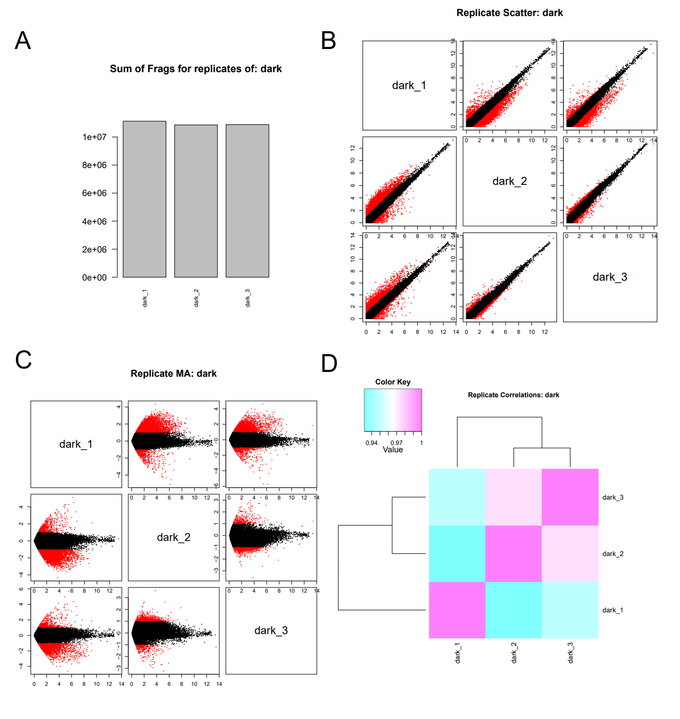
dark.rep_compare.pdf file. (A) The sum of mapped fragments. (B) Pairwise comparisons of replicate log(CPM) values, in which the data points more than 2-fold different are highlighted in red. (C) The pairwise MA plots (x-axis: mean log(CPM), y-axis log(fold_change)). And, (D) A Replicate Pearson correlation heatmap.6.3.2 Compare Replicates Across Samples
Activity
This command will generate a useful heatmap of pearson correlation matrix of samples from two different experimental groups.
PtR --matrix salmon.isoform.counts.matrix \
--min_rowSums 10 \
-s samples.txt \
--log2 --CPM \
--sample_cor_matrix
These files will append more to your current working directories:
-rw-rw---- 1 root PSLab    4012 Mar  6 15:02 salmon.isoform.counts.matrix.R
-rw-rw---- 1 root PSLab 3558147 Mar  6 15:02 salmon.isoform.counts.matrix.minRow10.CPM.log2.dat
-rw-rw---- 1 root PSLab     678 Mar  6 15:02 salmon.isoform.counts.matrix.minRow10.CPM.log2.sample_cor.dat
-rw-rw---- 1 root PSLab    6429 Mar  6 15:02 salmon.isoform.counts.matrix.minRow10.CPM.log2.sample_cor_matrix.pdf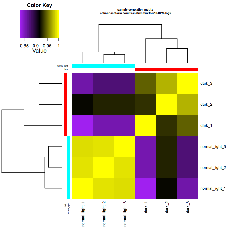
6.3.3 Principal Component Analysis (PCA)
Another important analysis method to explore relationships among the sample replicates is Principal Component Analysis (PCA).
You can find more explanation about PCA here: - https://blog.bioturing.com/2018/06/14/principal-component-analysis-explained-simply/ - https://youtu.be/FgakZw6K1QQ
Activity
PtR --matrix salmon.isoform.counts.matrix \
-s samples.txt \
--min_rowSums 10 --log2 \
--CPM --center_rows \
--prin_comp 3
These files will append more to your current working directories:
-rw-rw---- 1 root PSLab    4789 Mar  6 15:18 salmon.isoform.counts.matrix.R
-rw-rw---- 1 root PSLab 4069112 Mar  6 15:18 salmon.isoform.counts.matrix.minRow10.CPM.log2.centered.dat
-rw-rw---- 1 root PSLab     756 Mar  6 15:18 salmon.isoform.counts.matrix.minRow10.CPM.log2.centered.PCA.prcomp.scores
-rw-rw---- 1 root PSLab 4163653 Mar  6 15:18 salmon.isoform.counts.matrix.minRow10.CPM.log2.centered.PCA.prcomp.loadings
-rw-rw---- 1 root PSLab    5446 Mar  6 15:18 salmon.isoform.counts.matrix.minRow10.CPM.log2.centered.prcomp.principal_components.pdf
You can find the PCA plot in salmon.isoform.counts.matrix.minRow10.CPM.log2.centered.prcomp.principal_components.pdf.
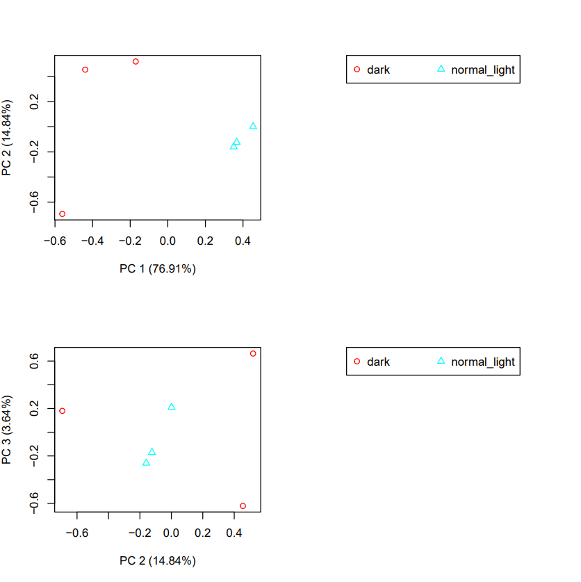
We set the number of principal components (PC) to be calculated for only first 3 PCs in --prin_comp. Which indicates that these PCs will be plotted, as shown above, with PC1 vs. PC2 and PC2 vs. PC3. In this example, the replicates cluster tightly according to sample type, which is very reassuring.
6.4 Differential Expression Analysis
Trinity also contains a built-in utility for DE analysis called run_DE_analysis.pl, in which use the count matrix and sample metadata file. Trinity provides support for several differential expression analysis tools, currently including edgeR, DESeq2, limma/voom, and ROTS.
DE analysis in Trinity will perform pairwise comparison of gene/transcript expression. If the biological replicates are presented for each sample, you should indicate this as we already created in our metadata table samples.txt. Here we’ll analyze DE genes in the ‘transcript’ level using the salmon.isoform.counts.matrix file.
Activity
DE analysis using DESeq2
run_DE_analysis.pl \
--matrix salmon.isoform.counts.matrix \
--method DESeq2 \
--samples_file samples.txt \
--output DESeq2_result
After run the above command, the following directory will append to your current working directory:
drwxrwx--- 1 root PSLab 688 Mar 6 15:42 DESeq2_resultIn this output directory, you’ll find the following files for each of the pairwise comparisons performed:
-rw-rw---- 1 root PSLab 972633 Mar 6 15:42 salmon.isoform.counts.matrix.dark_vs_normal_light.DESeq2.count_matrix
-rw-rw---- 1 root PSLab 4247784 Mar 6 15:42 salmon.isoform.counts.matrix.dark_vs_normal_light.DESeq2.DE_results
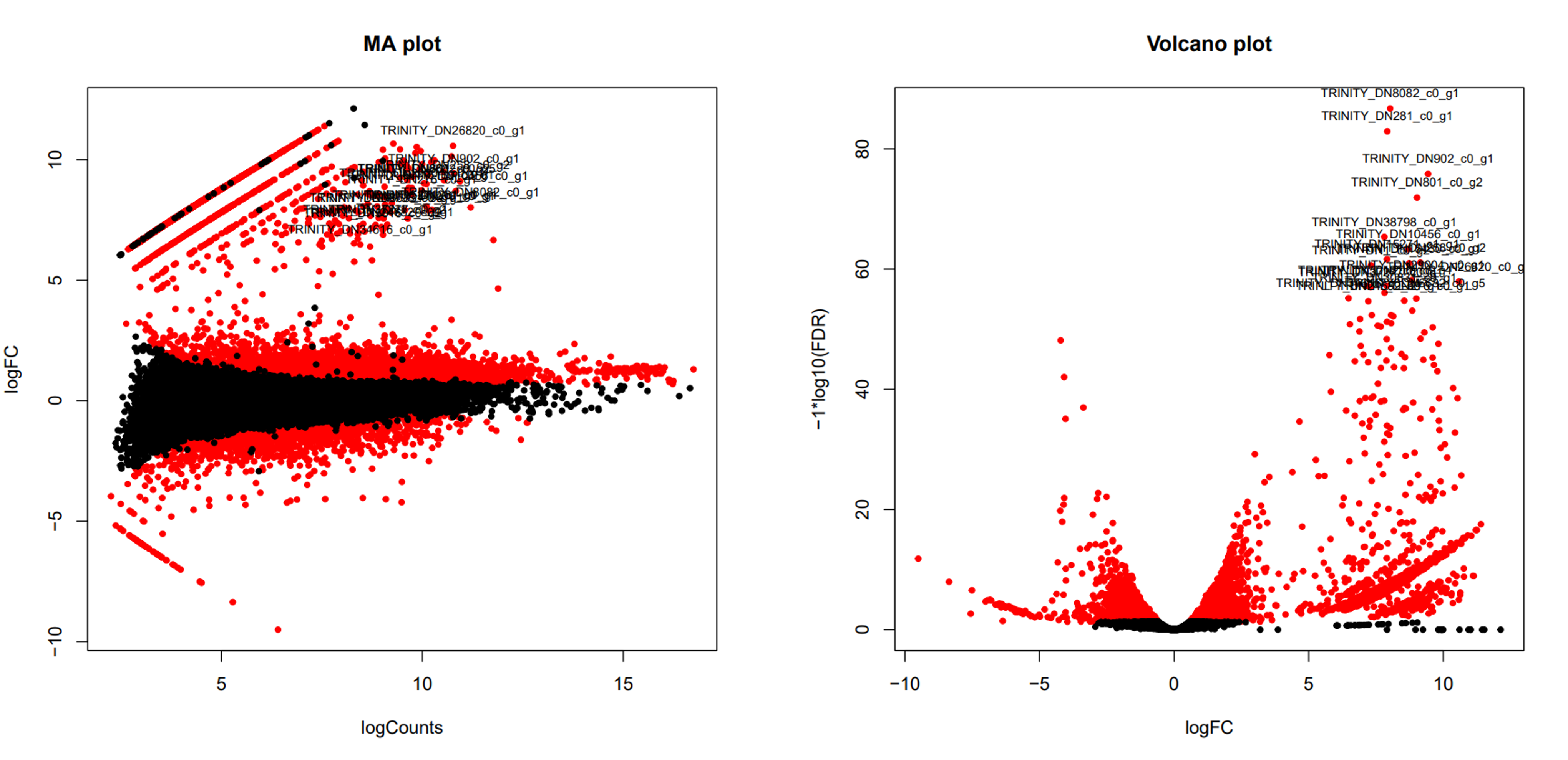
-rw-rw---- 1 root PSLab 2428272 Mar 6 15:42 salmon.isoform.counts.matrix.dark_vs_normal_light.DESeq2.DE_results.MA_n_Volcano.pdf
-rw-rw---- 1 root PSLab 1845 Mar 6 15:42 salmon.isoform.counts.matrix.dark_vs_normal_light.DESeq2.RscriptResult explanations:
salmon.isoform.counts.matrix.dark_vs_normal_light.DESeq2.Rscriptis the R-script executed to perform the DE analysis.salmon.isoform.counts.matrix.dark_vs_normal_light.DESeq2.count_matrixis an integer matrix of read count derived from the input filesalmon.isoform.counts.matrix.salmon.isoform.counts.matrix.dark_vs_normal_light.DESeq2.DE_resultsis the DE analysis results, including log fold change and statistical significance.salmon.isoform.counts.matrix.dark_vs_normal_light.DESeq2.DE_results.MA_n_Volcano.pdfis MA and Volcano plots features found DE at the defined FDR will be colored red.
Here’s an example of DE analysis result file (salmon.isoform.counts.matrix.dark_vs_normal_light.DESeq2.DE_results):
| sampleA | sampleB | baseMeanA | baseMeanB | baseMean | log2FoldChange | lfcSE | stat | pvalue | padj | |
|---|---|---|---|---|---|---|---|---|---|---|
| TRINITY_DN8082_c0_g1 | dark | normal_light | 4685.731 | 17.948650 | 2351.8401 | 8.023585 | 0.3947937 | 20.32349 | 0 | 0 |
| TRINITY_DN281_c0_g1 | dark | normal_light | 2406.185 | 9.827619 | 1208.0061 | 7.917578 | 0.3987747 | 19.85477 | 0 | 0 |
| TRINITY_DN902_c0_g1 | dark | normal_light | 3515.942 | 5.151569 | 1760.5469 | 9.433323 | 0.4966128 | 18.99533 | 0 | 0 |
| TRINITY_DN801_c0_g2 | dark | normal_light | 2100.468 | 4.052528 | 1052.2602 | 9.023139 | 0.4877916 | 18.49794 | 0 | 0 |
| TRINITY_DN38798_c0_g1 | dark | normal_light | 1013.842 | 4.511975 | 509.1769 | 7.806389 | 0.4421257 | 17.65649 | 0 | 0 |
| TRINITY_DN10456_c0_g1 | dark | normal_light | 3630.296 | 8.696336 | 1819.4963 | 8.698117 | 0.5004932 | 17.37909 | 0 | 0 |
| TRINITY_DN15271_c1_g1 | dark | normal_light | 1503.228 | 6.205016 | 754.7166 | 7.908525 | 0.4612383 | 17.14629 | 0 | 0 |
| TRINITY_DN258_c0_g2 | dark | normal_light | 2973.655 | 5.218821 | 1489.4370 | 9.144528 | 0.5358879 | 17.06425 | 0 | 0 |
| TRINITY_DN15130_c0_g1 | dark | normal_light | 2019.010 | 4.727083 | 1011.8685 | 8.728308 | 0.5121991 | 17.04085 | 0 | 0 |
| TRINITY_DN1_c0_g2 | dark | normal_light | 1107.861 | 6.860877 | 557.3612 | 7.312156 | 0.4304045 | 16.98903 | 0 | 0 |
An example of volcano plot for transcript-level differentially expression analysis.
6.5 Extracting and clustering differentially expressed transcripts
An initial step in analyzing differential expression is to extract those transcripts that are most differentially expressed (most significant FDR and fold-changes) and to cluster the transcripts according to their patterns of differential expression across the samples.
Activity
Extracting and clustering differentially expressed transcripts can run using the following from within the DE output directory, by running the following script:
cd DESeq2_result/
analyze_diff_expr.pl \
--matrix ../salmon.isoform.counts.matrix \
-P 1e-3 \
-C 2 \
--samples ../samples.txt \
--max_genes_clust 10000
The above command use an integer count matrix from DE analysis, and define criteria for extracting differentially expressed transcripts. For example, set p-value cutoff for FDR in -P to 0.001, set minimum absolute log 2-fold change criteria in -C to 2, meaning that it will extracted only the DE transcripts that are 2^2 = 4-fold, and use only top 10,000 among all differentially transcripts in --max_genes_clust for hierarchical clustering analysis. However, user can customize these criteria based on their interest.
The following results will append to the current working directory DESeq2_result
-rw-rw---- 1 root PSLab      120 Mar  6 16:34 salmon.isoform.counts.matrix.dark_vs_normal_light.DESeq2.DE_results.samples
-rw-rw---- 1 root PSLab   332012 Mar  6 16:34 salmon.isoform.counts.matrix.dark_vs_normal_light.DESeq2.DE_results.P0.001_C2.dark-UP.subset
-rw-rw---- 1 root PSLab    42038 Mar  6 16:34 salmon.isoform.counts.matrix.dark_vs_normal_light.DESeq2.DE_results.P0.001_C2.normal_light-UP.subset
-rw-rw---- 1 root PSLab   373901 Mar  6 16:34 salmon.isoform.counts.matrix.dark_vs_normal_light.DESeq2.DE_results.P0.001_C2.DE.subset
-rw-rw---- 1 root PSLab       51 Mar  6 16:34 DE_feature_counts.P0.001_C2.matrix
-rw-rw---- 1 root PSLab    73959 Mar  6 16:34 diffExpr.P0.001_C2.matrix
-rw-rw---- 1 root PSLab     4649 Mar  6 16:34 diffExpr.P0.001_C2.matrix.R
-rw-rw---- 1 root PSLab   246973 Mar  6 16:34 diffExpr.P0.001_C2.matrix.log2.centered.dat
-rw-rw---- 1 root PSLab      698 Mar  6 16:34 diffExpr.P0.001_C2.matrix.log2.centered.sample_cor.dat
-rw-rw---- 1 root PSLab     6399 Mar  6 16:34 diffExpr.P0.001_C2.matrix.log2.centered.sample_cor_matrix.pdf
-rw-rw---- 1 root PSLab   101250 Mar  6 16:34 diffExpr.P0.001_C2.matrix.log2.centered.genes_vs_samples_heatmap.pdf
-rw-rw---- 1 root PSLab 14777602 Mar  6 16:34 diffExpr.P0.001_C2.matrix.RData
Result explanations:
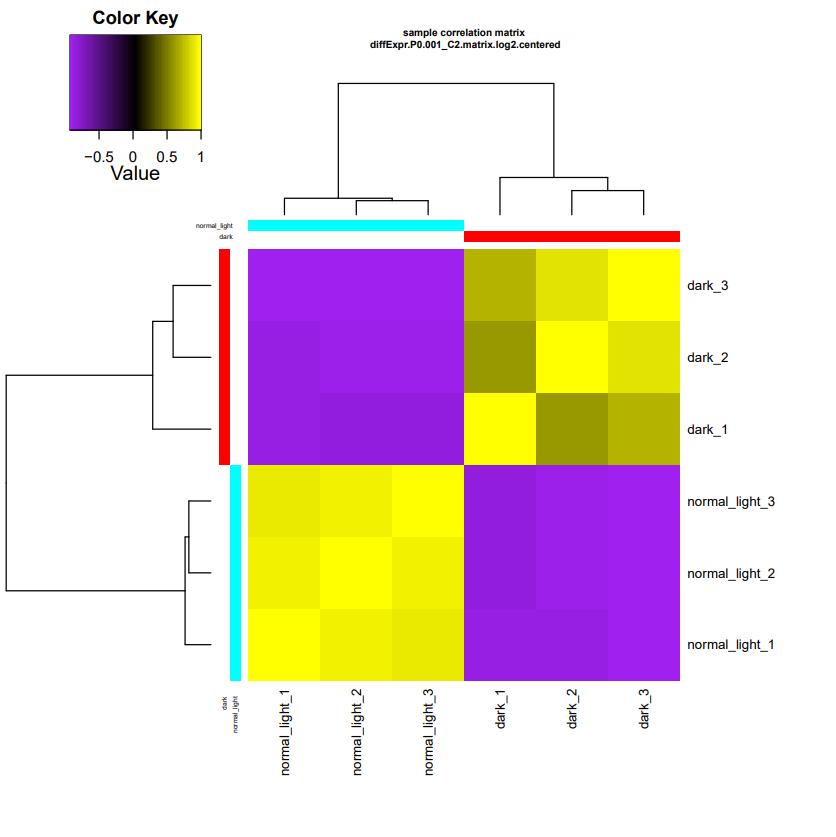
salmon.isoform.counts.matrix.dark_vs_normal_light.DESeq2.DE_results.samplesis identical to the metadatasamples.txtfile.salmon.isoform.counts.matrix.dark_vs_normal_light.DESeq2.DE_results.P0.001_C2.dark-UP.subsetis the subset of expression matrix of up-regulated transcripts in Dark group, which are down-regulated in Normal light group.salmon.isoform.counts.matrix.dark_vs_normal_light.DESeq2.DE_results.P0.001_C2.normal_light-UP.subsetis the subset of expression matrix of up-regulated transcripts in Normal light group, which are down-regulated in Dark group.salmon.isoform.counts.matrix.dark_vs_normal_light.DESeq2.DE_results.P0.001_C2.DE.subsetis a summary of DE transcripts results containing columns of significant values, and its normalized expression value.diffExpr.P0.001_C2.matrix.log2.centered.sample_cor_matrix.pdfis the sample correlation matrix, as follow.
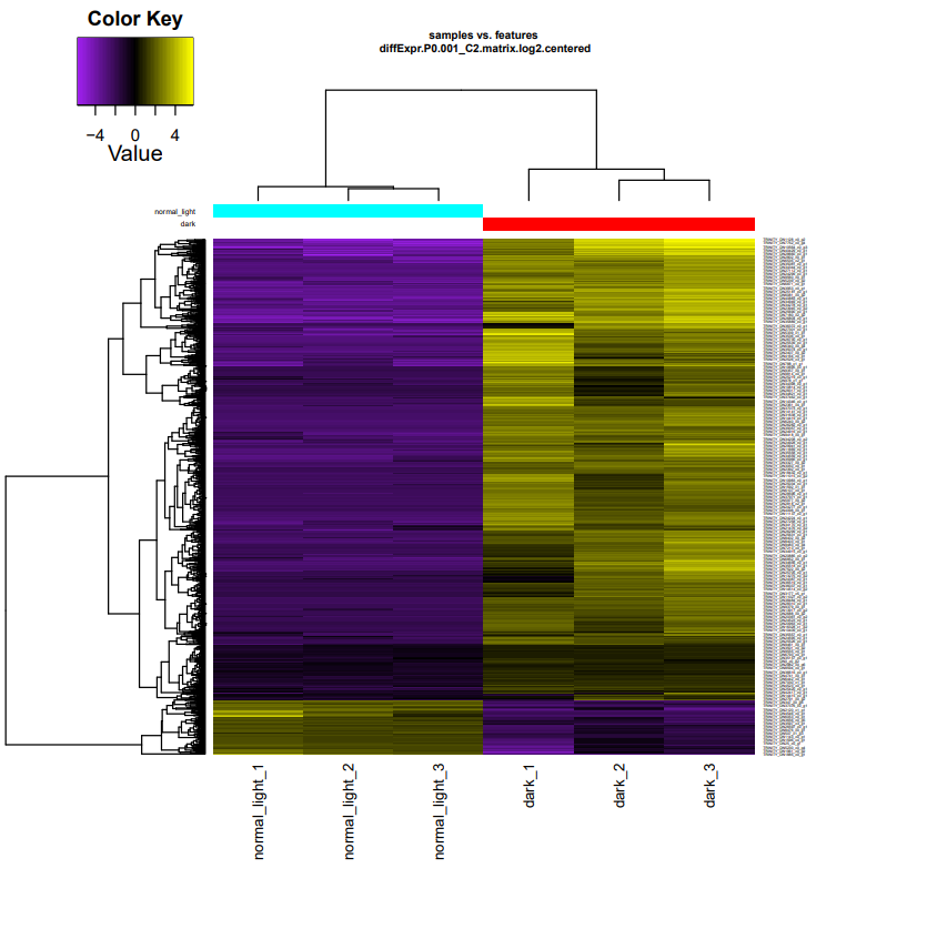
diffExpr.P0.001_C2.matrix.log2.centered.genes_vs_samples_heatmap.pdfis heatmap of differentially expressed transcripts.
6.6 DE gene patterning and clustering analysis
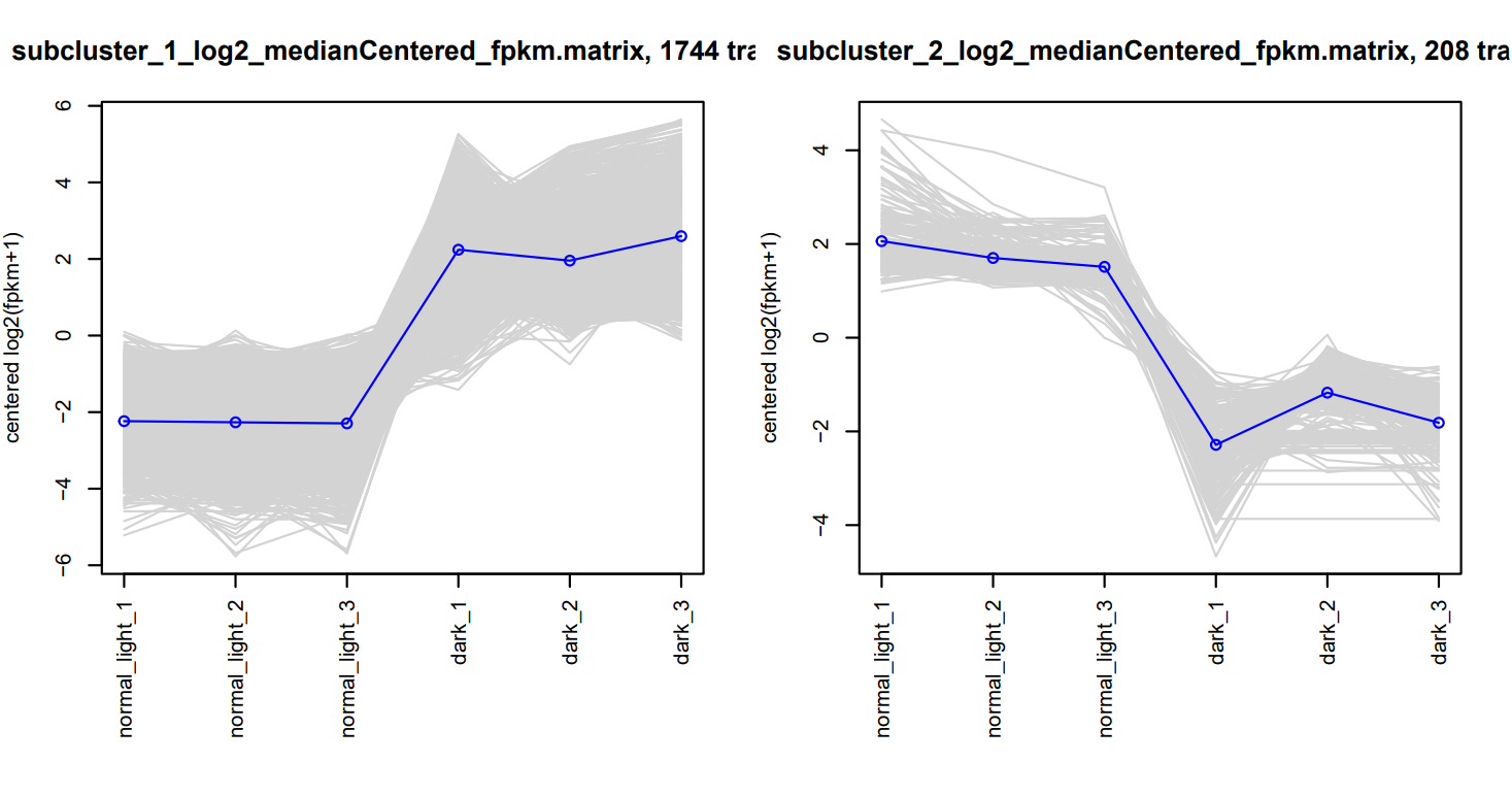
In the heat map of differentially expressed transcripts, there is a clear difference between the DE transcripts under dark and normal light conditions. Therefore, using define_clusters_by_cutting_tree.pl, we can divide these genes into clusters based on the same trend of expression values as follows.
Activity
Automatically Partitioning Genes into Expression Clusters
define_clusters_by_cutting_tree.pl \
-R diffExpr.*.matrix.RData \
--Ptree 60
There are three different methods for dividing genes into clusters, K-Means clustering, hierarchical clustering (as used in the heatmap), and the recommended method of using criteria to truncate tree branch lengths that fall below the criteria by using ‘–Ptree’.
The following results will append to the current working directory DESeq2_result which are files and diffExpr.P0.001_C2.matrix.RData.clusters_fixed_P_60/ directory.
-rw-rw---- 1 root PSLab    45837 Mar  6 16:51 clusters_fixed_P_60.heatmap.heatmap_gene_order.txt
-rw-rw---- 1 root PSLab    61467 Mar  6 16:51 clusters_fixed_P_60.heatmap.gene_cluster_colors.dat
-rw-rw---- 1 root PSLab   110890 Mar  6 16:51 clusters_fixed_P_60.heatmap.heatmap.pdf
drwxrwx--- 1 root PSLab      400 Mar  6 16:51 diffExpr.P0.001_C2.matrix.RData.clusters_fixed_P_60/
List of files in diffExpr.P0.001_C2.matrix.RData.clusters_fixed_P_60/ directory are:
-rw-rw---- 1 root PSLab  43915 Mar  6 16:51 my_cluster_plots.pdf
-rw-rw---- 1 root PSLab 220780 Mar  6 16:51 subcluster_1_log2_medianCentered_fpkm.matrix
-rw-rw---- 1 root PSLab  26259 Mar  6 16:51 subcluster_2_log2_medianCentered_fpkm.matrix
-rw-rw---- 1 root PSLab    816 Mar  6 16:51 __tmp_plot_clusters.R
The DE transcript partiitoning and clustering is located in my_cluster_plots.pdf
Then, we’ll subset the assembled transcriptome for only differentially expressed genes for functional annotation analysis in the next chapter.
Activity
From the previous command, we already have a list of differentialli expressed gnees in salmon.isoform.counts.matrix.dark_vs_normal_light.DESeq2.DE_results.P1e-3_C2.DE.subset file. For the functional annotation analysis in the next step, we will subset only top 10 upregulated and top 10 downregulated DEGs for annotation step. Data subsetting will use the following command.
- Extract top 10 upregulated DEGs in Normal light condition. This command will ascendingly sort the 6th column (log2foldchange) of the file
salmon.isoform.counts.matrix.dark_vs_normal_light.DESeq2.DE_results.P1e-3_C2.normal_light-UP.subset, then selected top 10 highest log2foldchange from the last 10 lines, then select only the trinity transcript ID in the first column.
sort --key=6 --numeric-sort salmon.isoform.counts.matrix.dark_vs_normal_light.DESeq2.DE_results.P1e-3_C2.normal_light-UP.subset | tail -n 10 | cut --fields=1 > DEGtop10_NormalLight-up.txt- Do the same for dark condiiton using
salmon.isoform.counts.matrix.dark_vs_normal_light.DESeq2.DE_results.P1e-3_C2.dark-UP.subsetfile.
sort --key=6 --numeric-sort salmon.isoform.counts.matrix.dark_vs_normal_light.DESeq2.DE_results.P1e-3_C2.dark-UP.subset | tail -n 10 | cut --fields=1 > DEGtop10_dark-up.txt- Concatenate transcript ID files (
DEGtop10_NormalLight-up.txtandDEGtop10_dark-up.txt) into a single file.
cat DEGtop10_NormalLight-up.txt DEGtop10_dark-up.txt > DEGtop20_all.txt- Retrieve FASTA sequence of top 20 DEGs using Trinity’s utility.
retrieve_sequences_from_fasta.pl DEGtop100_all.txt ~/Cpa_RNASeq/03_assembly/Trinity_2023-03-08.Trinity.fasta > DEGtop20_all_seqs.fastaThe output file locates in ~/Cpa_RNASeq/04_DE_analysis/DESeq2_result